22,580: From GPT-2 to Kimi K3 Seven Years of LLM Architecture Evolution, Explained
Twenty-two thousand five hundred eighty — that's how many GPT-2s (2019) fit inside one Kimi K3 (2026). In seven years, parameter counts ballooned by a factor of 22,580. But is this really just a story about "scale"? Starting from the five math building blocks a complete beginner needs, we walk the entire architectural path from GPT-2 to Kimi K3 — deriving every formula and reconciling every parameter count along the way.
Original: 22580: From GPT2 to Kimi3, Explained · ali (@waterloo_intern)This edition: English translation of the expanded Chinese rewrite (2nd edition)Reading time: ~90–120 minutes
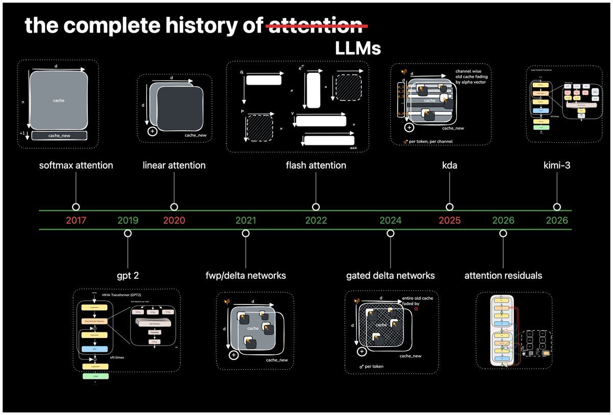
Original figureFrom GPT-2 to Kimi K3: the architectural journey this article walks in full.
Twenty-two thousand five hundred eighty.
That's the number of times GPT-2 (2019, ~124M parameters) fits inside Kimi K3 (2026, 2.8 trillion parameters). In seven years, we made models 22,580× bigger. But is the story really just "bigger"?
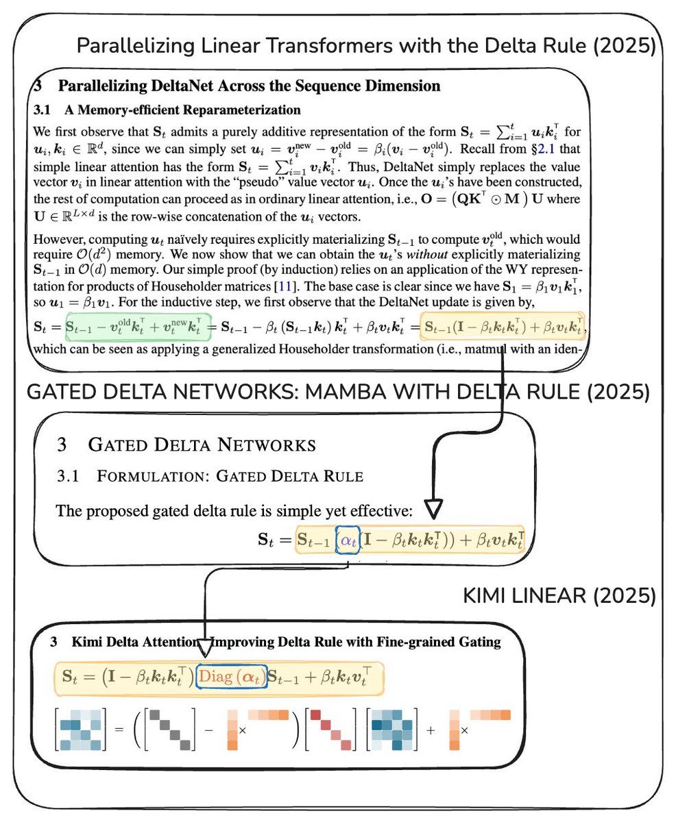
In this work-log-style long read, we trace step by step what actually happened over those years — you'll find that a great deal changed, and a surprising amount did not. The original author followed the linearization thread "linear attention → DeltaNet → Gated DeltaNet → Kimi Delta Attention" all the way to Kimi K3; this edition keeps that main thread intact (with all code and derivations) and adds a beginner-friendly math primer, worked-by-hand examples, parameter ledgers, and four side threads: the attention family (MQA/GQA/MLA), state space models (Mamba), MoE sparsity, and training/inference optimization. By the end, someone who knows almost nothing about LLMs can assemble the full knowledge map — the kind where you can actually do the math.
HOW TO READ THIS
The article has four kinds of content: the primer (01) fills in every mathematical prerequisite for beginners, computing each building block by hand; the main-thread chapters (02, 04–06, 08, 09, 11, 12) translate and explain the original's architecture evolution chain; the interlude chapters (03, 07, 10, 13) are new background material; 14, 15, and Appendices A/B hold the timeline, the conclusion, and complete proofs. All code runs as-is, and every formula comes with intuition or a step-by-step derivation. If you already know Transformer basics, you can start directly at Chapter 02.
LLM papers look formula-heavy, but only five building blocks get used over and over: vectors, dot products, matrix multiplication, Softmax, and logarithms. We'll compute each one by hand — something you've computed by hand is something you've truly learned.
1.1 Building blocks one through five, each computed by hand
Block 1: A vector isn't "one meaning" — it's a set of coordinates
Why does one token become thousands of numbers? Because a single scalar can't simultaneously express "part of speech, semantics, tone, entity, position" and dozens of other attributes. The model gives each token a \(d\)-dimensional vector; individual dimensions need not have human-nameable meanings — information is usually distributed across combinations of many dimensions.
A two-dimensional toy representation2-D TOY EMBEDDING
Add the products\(6 + (-4) = 2\), so \(q \cdot k = 2\).
Geometric reading\(q \cdot k = \|q\|\,\|k\|\cos\theta\). With lengths fixed, closer directions give larger dot products; opposite directions give negative ones.
WHY THIS WORKS AS RETRIEVAL
Encode what the current token needs as a query \(q\), and the retrievable label of every past token as a key \(k\). The bigger the dot product, the more of the corresponding value gets read. Note: this matching space is learned by training, not hand-specified keyword matching.
Block 3: Matrix multiplication is "dot products in bulk"
If \(A\) is \(m \times n\) and \(B\) is \(n \times p\) (the inner \(n\) must match), the product \(AB\) is \(m \times p\). Entry \((i,j)\) of the result is the dot product of row \(i\) of A with column \(j\) of B.
Block 4: Softmax turns arbitrary scores into probabilities
Why not use the dot-product scores directly as weights?
Dot products can be negative and have no fixed sum. Softmax first exponentiates to make every term positive, then divides by the total so all weights sum to 1: \(p_i = e^{z_i} / \sum_j e^{z_j}\).
Divide each by Z\(p \approx [0.665,\ 0.245,\ 0.090]\), which conveniently sums to ~1.
Numerical-stability trick: \(\text{softmax}(z) = \text{softmax}(z - \max(z))\). Subtracting 2 from every score gives \([0,-1,-2]\) — the probabilities are unchanged, but you avoid computing overflow-prone huge exponentials. FlashAttention generalizes exactly this trick to chunked computation (see §3.4 and the full proof in Appendix A).
Block 5: Logarithms turn "small probability" into "large penalty"
If the correct answer has probability \(p\), the cross-entropy loss is \(-\log p\). The more confident and correct the prediction, the closer the loss is to 0; the smaller the probability on the right answer, the larger the loss:
Probability p on correct answer
Loss −ln p
Intuition
0.90
0.105
Confidently right, small penalty
0.50
0.693
A coin flip
0.10
2.303
Correct answer pushed down hard, big penalty
0.001
6.908
Extremely confident about ignoring the right answer
Why is Softmax + cross-entropy so optimization-friendly?THE KEY GRADIENT
Let the logits be \(z\), the Softmax probabilities \(p\), and the correct class \(y\). Differentiating the combined loss gives a remarkably clean result:
\(\mathbb{1}[i=y]\) means: 1 if \(i\) is the correct answer, else 0. Reusing \(p=[0.665, 0.245, 0.090]\) above and supposing the second class is correct, the gradient is \([0.665, -0.755, 0.090]\). Gradient descent will push down the scores of classes one and three and push up class two. This isn't a vague "the model knows it was wrong" — every logit receives a computable direction of change. This elegant gradient is the bedrock of the entire LLM training edifice.
1.2 What "predicting the next token" actually optimizes
The training objective of GPT-style models is disarmingly plain: given the preceding tokens, raise the probability of the true next token. Complex abilities don't come from a separate "understand the world" loss — they emerge gradually from compressing the regularities of massive sequences.
First, shift a sentence by one position
Input 〈BOS〉 → I → love → cats
→
Model forward each position sees only its left
→
Target I → love → cats → 〈EOS〉
During training, all four positions can compute their losses simultaneously (this is why GPU-parallel training works); but each position may only look at itself and to its left — never peek at the target on its right. This constraint is enforced by the "causal mask" of Chapter 02.
The first line factorizes the probability of the whole text into per-step conditionals via the chain rule; the second takes the negative log, turning "maximize a product" into "minimize a sum," which is numerically friendlier.
Why doesn't the model just memorize the training text?
It does memorize some frequent or repeated content, but parameter capacity, data scale, and the training process force the model to reuse regularities massively. Completing "Paris is the capital of ___" requires entity relations; completing code requires syntax and variable dependencies; completing a proof requires reasoning patterns. Next-token prediction is the objective — it doesn't mean the internals can only learn a word-level lookup table.
More precisely, the model learns a conditional probability distribution. At generation time we greedily take the argmax or sample with temperature from that distribution.
From token id to probabilities: the complete pipeline
token id integer
→
Embedding token → vector
→
Attention / KDA mixing across tokens
→
MLP / MoE transform within each token
→
Vocab projection vector → probabilities
A master map: every layer does only two kinds of mixing — attention-like modules move information between tokens (across positions), and MLP-like modules transform information within each token (within a position). Every architecture innovation in the rest of this article is a replacement for what sits inside these two boxes.
# batch dim omitted; T = sequence length, d = hidden dim, V = vocab size
X = Embedding[token_ids] # [T] → [T, d]for layer in layers:
X = X + Attention(RMSNorm(X)) # mixing across tokens
X = X + MLP(RMSNorm(X)) # transform within each token
logits = RMSNorm(X) @ W_vocab.T # [T,d]×[d,V] → [T,V]
prob = softmax(logits, axis=-1) # each row becomes a vocab distribution
loss = -mean(log(prob[true_next_token]))
Is Embedding some mysterious algorithm?
No. It is first and foremost a trainable table \(E \in \mathbb{R}^{V \times d}\). If the token id is 17, you take row 17. If you write the id as a one-hot vector with a single 1, the lookup is equivalent to a matrix multiply — it's just that engineering-wise nobody actually materializes the giant one-hot.
Residual connections and normalization: stabilizers for deep networks
\[
u = x + \text{Attention}(\text{RMSNorm}(x)), \qquad
y = u + \text{MLP}(\text{RMSNorm}(u))
\]
If a new branch \(F\) hasn't learned anything useful yet, the model can still pass information and gradients along the "+x" express lane; deep networks are therefore much easier to train. This is the famous Pre-Norm residual structure.
By hand, RMSNorm: x = [3, 4], with g = [1,1], ε = 0NORMALIZATION
\(\text{RMS}(x) = \sqrt{\frac{1}{d}\sum_j x_j^2 + \epsilon}\), \(\quad \text{RMSNorm}(x) = g \odot x / \text{RMS}(x)\)
\(\text{RMS} = \sqrt{(3^2 + 4^2)/2} = \sqrt{12.5} \approx 3.536\), so the normalized vector is roughly \([0.849,\ 1.131]\). It doesn't point every vector in the same direction — it just pulls the overall scale back into a stable range; the trainable gain \(g\) then decides how large each dimension should be.
The MLP: two (or three) linear transforms
The original GPT-2 used a two-layer MLP: expand from \(d\) to \(d_{ff}\), apply GELU, project back to \(d\). Modern models mostly use the three-way SwiGLU structure:
\[
g = \text{SiLU}(xW_{gate}),\quad u = xW_{up},\quad \text{MLP}(x) = (g \odot u)\, W_{down}
\]
\(\odot\) is element-wise multiplication. The gate branch decides which expanded dimensions pass through, the up branch supplies content, and down projects back to model width. Ignoring biases, the three weight matrices hold \(d \times d_{ff}\), \(d \times d_{ff}\), and \(d_{ff} \times d\) parameters — about \(3 d d_{ff}\) in total. This single formula will later explain exactly where Kimi K3's trillion parameters come from (full reconciliation in §11.2).
Training objective = maximize the probability of the true next token at every position; the Softmax+cross-entropy gradient is \(p - \mathbb{1}[y]\), remarkably clean.
Master map: each layer = one across-token mixing (attention) + one within-token transform (MLP), with residuals and normalization as escorts.
02Ground Zero: Dissecting GPT-2
GPT-2 · 2019 · DECODER-ONLY TRANSFORMER
To understand every improvement that follows, we must first strip the baseline model to the bone. GPT-2 is a canonical decoder-only architecture — nearly every mainstream LLM today (GPT, Llama, Qwen, DeepSeek, Kimi) belongs to this family. Its entire forward pass fits in under 15 lines of code:
2.1 From embeddings to output: one complete forward pass
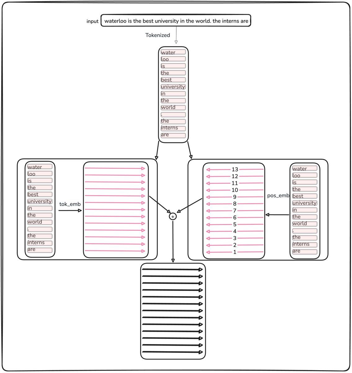
The input text is first split by a tokenizer into a token sequence (GPT-2 uses BPE, vocab ≈ 50,257). Each token looks up a 768-dim vector (token embedding), and the vector of its position is added (position embedding) — note that GPT-2's positional encoding is a learned absolute position embedding, a trainable lookup table just like the token embedding. This would later be completely overhauled (see §3.2).
Original figureToken and position embeddings are added to form the model's initial input representation. The figure also shows an important fact: only the logits at the final position are used to predict the next token.
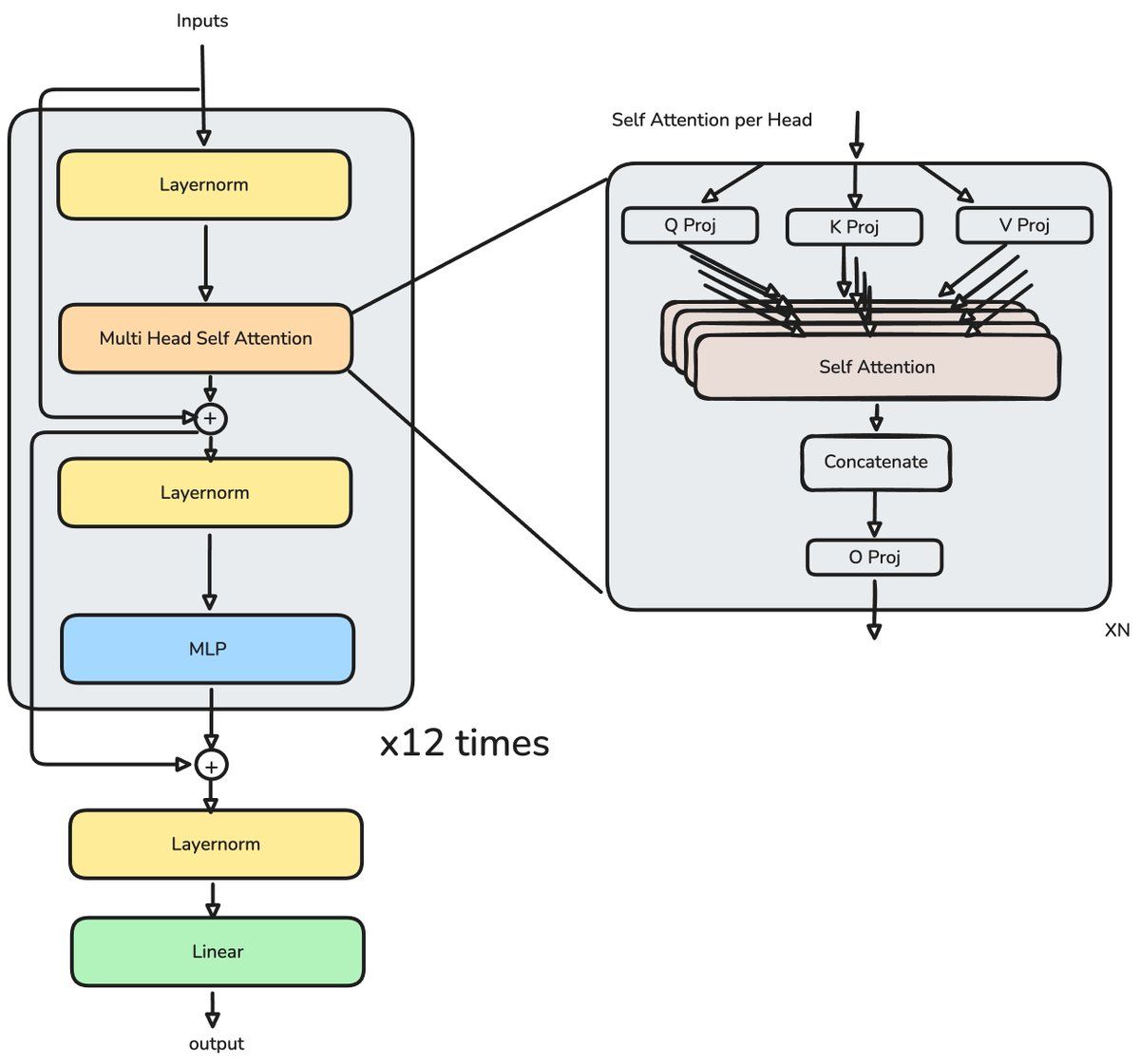
After the embeddings are added, the data flows through 12 structurally identical Transformer blocks. Zooming into one block:
classBlock(nn.Module):
def__init__(self, config):
super().__init__()
self.ln_1 = LayerNorm(config.n_embd, bias=config.bias)
self.attn = CausalSelfAttention(config)
self.ln_2 = LayerNorm(config.n_embd, bias=config.bias)
self.mlp = MLP(config)
defforward(self, x): # x: (b, t, n_embd)
x = x + self.attn(self.ln_1(x)) # attention sublayer + residual → (b, t, n_embd)
x = x + self.mlp(self.ln_2(x)) # MLP sublayer (up to 4×n_embd, then back) → (b, t, n_embd)return x # (b, t, n_embd)
Original figureA single GPT-2 Transformer block: LayerNorm → attention → residual add → LayerNorm → MLP → residual add. This "sandwich" structure has barely changed in seven years — what changed is which attention mechanism and which MLP sit inside.
BACKGROUND CARD · WHY RESIDUAL CONNECTIONS MATTER
Notice the pattern x = x + f(x). It lets each layer learn only a "correction to the input" rather than a whole new representation, and gradients flow back along the identity path without degradation, so networks tens or hundreds of layers deep train stably. The 2017 original Transformer placed LayerNorm after each sublayer (Post-LN); starting with GPT-2 it moved before each sublayer (Pre-LN), greatly improving deep-model training stability — an ordering still used today. And the residual itself gets reinvented again in Chapter 12 (AttnRes).
2.2 Causal attention, computed by hand
The heart of each block is Causal Self-Attention. Its code is startlingly short too:
B, T, C = x.size() # batch, sequence length, embedding dim; x: (B, T, C)# one linear projection computes q, k, v at once, then split into heads
q, k, v = self.c_attn(x).split(self.n_embd, dim=2) # (B,T,C)→(B,T,3C), split into three (B, T, C)
k = k.view(B, T, self.n_head, C // self.n_head).transpose(1, 2) # (B, nh, T, hs)
q = q.view(B, T, self.n_head, C // self.n_head).transpose(1, 2) # (B, nh, T, hs)
v = v.view(B, T, self.n_head, C // self.n_head).transpose(1, 2) # (B, nh, T, hs), hs = C/nh is head dim# attention scores: each query dotted with all keys, divided by √d_head
att = (q @ k.transpose(-2, -1)) * (1.0 / math.sqrt(k.size(-1))) # (B,nh,T,hs)×(B,nh,hs,T) → (B, nh, T, T)
att = att.masked_fill(self.bias[:,:,:T,:T] == 0, float('-inf')) # causal mask, (B, nh, T, T)
att = F.softmax(att, dim=-1) # (B, nh, T, T), each row sums to 1
y = att @ v # (B,nh,T,T)×(B,nh,T,hs) → (B, nh, T, hs)
y = y.transpose(1, 2).contiguous().view(B, T, C) # reassemble heads → (B, T, C)
y = self.resid_dropout(self.c_proj(y)) # output projection → (B, T, C)return y
Condensed into a formula:
\[
\text{Attention}(Q,K,V) = \text{softmax}\!\left(\frac{QK^\top}{\sqrt{d_h}} + M\right)V
\qquad
Q = XW_Q,\; K = XW_K,\; V = XW_V
\]
Rather than memorizing the formula, let's actually compute one pass. Suppose the projections have produced Q/K/V for three tokens (2-dim, single head). We only want the output of token 3, i.e. we dot \(q_3 = [0,1]\) with each of the three keys:
Position
q (only q₃)
k
v
q₃·k / √2
1
[1, 0]
[1, 0]
[1, 0]
0/√2 = 0
2
[1, 1]
[1, 1]
[0, 2]
1/√2 ≈ 0.707
3
[0, 1]
[0, 1]
[1, 1]
1/√2 ≈ 0.707
From scores to output, no steps skippedONE ATTENTION ROW
The attention output is not "picking one word" — it is usually a continuous weighted blend of several values. The weights are determined by the current query, so the same history returns different results for different queries.
The causal mask: no peeking at the future, even in training
For row \(t\), only positions \(1 \dots t\) are visible. Scores at future positions get \(-\infty\) added, which Softmax turns into weight 0:
This lets training compute all positions in parallel while preserving the same information constraint as token-by-token generation. What runs in parallel is the matrix math — early positions never see the future. This is the mathematical guarantee of "autoregressive generation," and the dividing line between decoder-only models and BERT-style encoders.
Why divide by √d_h? Is that scaling just a guess?
No. Suppose the dimensions of q and k are independent with mean 0 and variance 1; then each product \(q_j k_j\) has variance ≈ 1. Summing d terms, the dot product has variance ≈ \(d\), standard deviation ≈ \(\sqrt{d}\). The larger the dimension, the more extreme the unscaled logits, and the more Softmax saturates into near one-hot — gradients vanish. Dividing by \(\sqrt{d}\) brings the variance back to ≈ 1, keeping the numeric scale stable at any head dimension.
Multiple heads are not computing the same thing repeatedly
Each head has its own projection matrices, so it can learn a different matching subspace (syntax, coreference, positional proximity, etc.). With total hidden dim \(d = h \cdot d_h\), concatenation returns to d dimensions, and \(W_O\) then mixes the heads. The number and organization of heads becomes the protagonist of Chapter 03.
Where the quadratic complexity comes from
\(QK^\top\) produces a \(T \times T\) score matrix: each of T queries compares with each of T keys, each dot product costs ≈ d, so the rough compute is \(O(T^2 d)\), and storing the attention weights explicitly is \(O(T^2)\). Feel the horror of "quadratic" in this table:
Sequence length T
Number of attention scores T²
Relative to 4K
4,096
16,777,216
1×
32,768
1,073,741,824
64×
1,048,576
1,099,511,627,776
65,536×
AN IMPORTANT DISTINCTION
FlashAttention (§3.4) avoids writing the full T×T matrix back to HBM, making computation faster and far more memory-efficient — but it still computes exact Softmax attention; the arithmetic complexity remains quadratic. Linear attention in Chapter 04, by contrast, genuinely rewrites the mathematical structure. One route changes the engineering, the other changes the math — don't confuse them.
2.3 KV Cache: the first engineering compromise
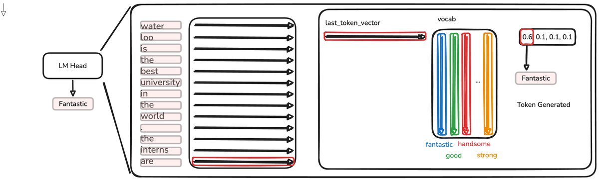
After the last Transformer block outputs the hidden-state matrix, the language model head (LM head) maps it to vocab-sized logits. In autoregressive decoding, each step needs only the logits at the last position to sample the next token.
This exposes a natural inefficiency of decoder-only generation: the model computes full representations for every input position, yet each decoding step consumes only the last position's logits. Without any caching, generating the next token would redo all of that computation verbatim.
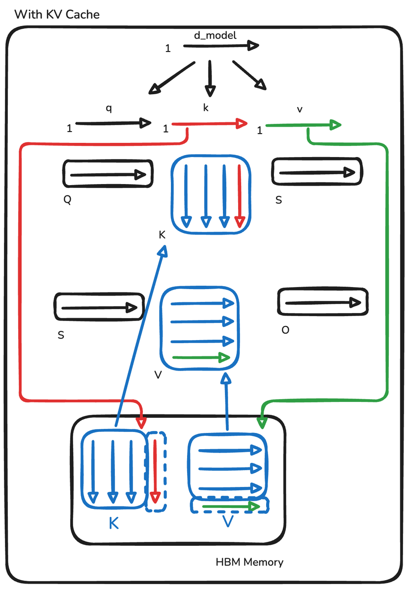
KV Cache comes from a plain observation: after appending the newly generated token to the input, the key and value projections of all previous tokens are bit-for-bit identical — the causal mask guarantees that past representations are unaffected by the future. So store their K and V vectors; the next step only needs to compute QKV for the new token and attend against every cached K and V. Compute per step drops from \(O(N^2)\) to \(O(N)\).
Original figureDecoding with KV Cache: each step computes Q/K/V only for the new token; historical K/V is reused directly. The price is a cache in GPU memory that grows linearly with the sequence.
That storage is the KV Cache. It keeps the K/V vectors of the previous \(N-1\) tokens, at \(2 \times N \times n_{layer} \times n_{head} \times d_{head} \times 2\) bytes (FP16), growing linearly with sequence length — quickly large enough to turn inference into a memory-bandwidth bottleneck rather than a compute bottleneck. Remember this sentence: from GQA to MLA to linear attention, almost the entire evolutionary line that follows is a war against "KV Cache too big."
Isn't the KV cache constantly being "updated"? Why say every token gets its own copy stored?
This is an especially confusing point: the KV Cache is a ledger — append-only, never updated. When token 1 is generated, the cache holds 1 K/V pair; when token 100 is generated, it holds 99 pairs — not one pair fewer; generate one more and it appends to 100 pairs. No pair is ever overwritten or merged.
Why can't pairs be merged? Because the next attention step must "take my new query and dot it individually with every key in history to decide whose value to read." If tokens 37 and 58 had their K/V merged, the model could never tell them apart again — and "every token keeps an independent slot, retrievable with precision at any time" is exactly the foundation of standard attention's quality.
Do the math: in GPT-2, each historical token stores 12 layers × 12 heads × 2 (K and V) × 64 dims × 2 bytes ≈ 36 KB. Every extra token of sequence eats another 36 KB — one more copy per token, not one copy total. In a modern large model (80 layers, 128-dim heads), it's ~0.3 MB per token, so a single 128K-context request needs ~40 GB of cache — that's the "memory explosion."
What truly has "update" semantics is the state \(S\) of Chapter 04's linear attention (S = S + k @ v): all history is folded into one fixed-size matrix, where old information gets overwritten and interfered with by new information — that's the "whiteboard." The contest between these two memory philosophies is the main thread of this article:
Standard attention KV Cache (ledger)
Linear-attention state S (whiteboard)
Structure
One independent slot per token (a list)
All tokens share one fixed matrix
Operation
Append only, never overwrite
Update only (accumulate/rewrite), never grows
Retrieval
Precise (can single out token 37)
Blurry (history mutually aliased)
Memory
Grows linearly with sequence — explodes
Constant, tiny
Representatives
GPT-2, Llama (compressed via GQA/MLA)
Linear attention, DeltaNet, KDA (Ch. 04–09)
From MQA/GQA (store fewer copies) to MLA (compress each copy) to linear attention (drop the list entirely) — seven years of architecture innovation has been a search for balance points between the two ends of this table.
2.4 The parameter ledger: where 124M comes from
"Parameters" are the numbers updated during training and read during inference. Once you see the shape of every weight matrix, parameter counts stop being a mysterious vendor total and become an addition problem you can audit. A dense Transformer has four ledgers:
Module
Main matrices
Parameters (ignoring bias)
Grows with
Token embedding
\(E \in \mathbb{R}^{V \times d}\)
\(Vd\)
Vocab V, width d
Attention
\(W_Q, W_K, W_V, W_O\), each ≈ d×d
\(4d^2\)
Width squared
GPT-2-style MLP
d→d_ff→d
\(2dd_{ff}\)
Width × intermediate dim
SwiGLU MLP
gate, up, down matrices
\(3dd_{ff}\)
Width × intermediate dim
Normalization
Per-dim scale (some with bias)
\(O(d)\)
Relatively small
Why does doubling model width usually more than double the parameters?
Because the main matrices contain d on both sides. A \(d \times d\) matrix becomes \((2d)^2 = 4d^2\) when d doubles; if the layer count doubles too, trunk parameters grow roughly 8×. Parameter scaling is about matrix area, not vector length.
Position embedding\(1{,}024 \times 768 = 786{,}432\).
Attention weights per layer\(4 \times 768^2 = 2{,}359{,}296\).
MLP weights per layer\(2 \times 768 \times 3{,}072 = 4{,}718{,}592\).
Main weights across 12 layers\(12 \times (2{,}359{,}296 + 4{,}718{,}592) = 84{,}934{,}656\).
Total\(38.60\text{M} + 0.79\text{M} + 84.93\text{M} \approx 124.3\text{M}\), plus ~0.12M of bias and LayerNorm, giving ≈ 124.44M. The output vocab projection shares weights with the token embedding, so we don't add another 38.6M.
Original figureVisualization of GPT-2's parameter breakdown. Note that the MLP holds about two-thirds of the parameters — which explains why MoE later chose to operate on the MLP (Chapter 10).
Total: ~124 million parameters. Kimi K3 has 2.8 trillion — one K3 holds about 22,580 GPT-2s.
Original figureA 22,580× gap in parameter scale. But as the rest of this article shows, the difference is far more than a number — what is stored, how it is updated, and how it is retrieved have all been redesigned.
The original's main thread jumps straight into "linear attention," but before that, industry actually took another path first: don't change attention's math — change its storage and engineering. This side thread gave us GQA, RoPE, RMSNorm, and FlashAttention, standard equipment in every mainstream model today. We must fill it in.
3.1 MHA → MQA → GQA → MLA: the siege on KV Cache
GPT-2 uses Multi-Head Attention (MHA): 12 heads, each with its own independent Q, K, V. The problem is the KV Cache — every head must store a K and a V for every historical token. 12 layers × 12 heads × 2 (K and V) × 64 dims × per token — memory explodes on long sequences.
The evolutionary chain is textbook-clear:
MQA (Multi-Query Attention, Shazeer 2019): all query heads share a single K and V. The KV Cache is divided by the head count (12× compression), decoding throughput jumps — but with a perceptible quality loss.
GQA (Grouped-Query Attention, 2023, popularized by Llama 2): the compromise — split Q heads into groups, each group sharing one K/V. Llama 2 70B uses \(h=64\) Q heads with \(g=8\) KV groups, compressing the cache 8× with almost no quality loss. GQA then became the default for 2023–2024 open models (Llama, Qwen, Mistral).
MLA (Multi-head Latent Attention, DeepSeek-V2, 2024): a different idea — instead of sharing K/V, jointly low-rank compress all heads' K/V into a small latent vector, store that, and decompress on use. Higher compression than GQA, and paradoxically better quality. This is core technology of DeepSeek-V2/V3 and the Kimi family; §10.2 dissects it in detail.
Figure 3-1 (self-drawn): the siege on attention's KV Cache. Orange = Query heads, green = the K/V that must be cached per token, yellow = MLA's compressed latent vector.
Mechanism
Introduced
KV cache per token
Quality
Representative models
MHA
2017
\(2 \cdot n_{head} \cdot d_h\)
Baseline
GPT-2/3, original Transformer
MQA
2019
\(2 \cdot d_h\) (÷ head count)
Slightly worse
Falcon, early PaLM
GQA
2023
\(2 \cdot n_{group} \cdot d_h\)
≈MHA
Llama 2/3QwenMistral
MLA
2024
\(d_c + d_h^R\) (latent dims, 90%+ compression)
Beats MHA
DeepSeek-V2/V3Kimi K2/K3
3.2 Position encoding: the victory of RoPE
GPT-2 uses learned absolute position embeddings, with two hard flaws: the longest sequence seen in training is the capability ceiling, and position information is entangled with content information. The evolutionary path:
Sinusoidal encoding (original 2017 Transformer): generated by a fixed formula, no learning needed, slightly better extrapolation — still fragile.
RoPE (Rotary Position Embedding, Su Jianlin 2021): encode position as a rotation of 2-D subspaces of the Q/K vectors — the query at position \(m\) is rotated by \(m\theta\). All of Llama, Qwen, DeepSeek, and Kimi use RoPE, one of the few "zero-controversy" technical consensuses of recent years.
Length-extrapolation patches: RoPE fails when extrapolated directly beyond trained lengths, so a family of "length-extension" techniques appeared — Position Interpolation, NTK-aware scaling, YaRN — letting a 4K-trained model serve 128K or longer.
ALiBi (2022): instead of adding position to embeddings, add a distance-proportional penalty directly to attention scores; excellent extrapolation (adopted by BLOOM).
NoPE / emergent causal position: another interesting finding — decoder-only models learn some position sense even with no position encoding at all; and the linear-attention/RNN architectures of Chapter 04 have position built into the recurrence by construction.
Deriving RoPE: make the dot product depend only on relative positionROTARY DERIVATION
Goal: find a position encoding such that the inner product of \(q_m\) and \(k_n\) depends only on the relative position \(m-n\):
Key identity: rotation matrices satisfy \(R(m\theta)^\top R(n\theta) = R((n-m)\theta)\), so
\[ \big(R(m\theta)q\big)^\top \big(R(n\theta)k\big) = q^\top R\big((n-m)\theta\big)\, k \]
The dot product naturally depends only on the relative distance \(n-m\). Generalizing to d dimensions (even), pair up the dimensions and give each pair its own rotation frequency \(\theta_i = 10000^{-2i/d}\): high-frequency pairs handle nearby structure, low-frequency pairs handle distant structure — position is encoded directly in vector rotation, no additive position embedding needed, and attention decays naturally with distance.
3.3 Normalization and activations: the quiet foundation
These changes aren't sexy, but each one saved real money:
LayerNorm vs RMSNorm: half the computation you can throw awayNORMALIZATION
Why can the mean go? Experiments show re-centering barely affects performance, and dropping it cuts normalization compute by roughly 10–20%. Normalization appears twice per Transformer layer, so the saving is substantial — after Llama, RMSNorm became the de facto standard.
Component
Old
New
Why switch
Normalization
LayerNorm (subtract mean, divide std)
RMSNorm (divide RMS only)
No mean shift, ~10–20% less compute, no quality loss
Norm position
Post-LN
Pre-LN
Stable deep training, no tricky warmup; pioneered by GPT-2
Stability patches
—
QK-Norm, z-loss, sandwich norm
Prevents attention logits and residual-stream blowups (echoed by AttnRes in Ch. 12)
FFN activation
ReLU / GELU
SwiGLU: \((xW_1 \odot \text{SiLU}(xW_g))W_2\)
Gated linear unit, better at equal params; hidden dim set to \( \frac{8}{3}d \) to match parameter count
FFN structure
Expand → activate → contract
Gated three-way
Established by PaLM/Llama; SiTU in Ch. 11 is a distant cousin
3.4 FlashAttention: same math, new world
Tri Dao's FlashAttention (2022) is perhaps the single most industry-impactful paper of the era. It changed nothing about attention's mathematical definition — its output is bit-equivalent to the standard implementation. What it changed is how the computation is organized on the GPU.
The key insight: the bottleneck of standard implementations is not FLOPs but memory IO. A naive implementation materializes the full \(N \times N\) attention-score matrix to HBM (high-bandwidth memory), reads it back for softmax, writes it back, reads it again to multiply by V — at 8K sequence length that intermediate matrix is already several GB. GPU SRAM (on-chip cache) is an order of magnitude faster but tiny (~200KB per SM). FlashAttention's approach:
Tiling: cut Q/K/V into blocks that fit in SRAM;
Online softmax: while sweeping K/V blocks, maintain a running maximum and normalization factor, completing exact softmax in one pass — the \(N \times N\) matrix is never materialized;
Recomputation: in backprop, don't store the attention matrix — recompute it on demand. More FLOPs, less IO, faster overall.
The online Softmax algorithm: FlashAttention's most elegant stepONLINE SOFTMAX
Standard Softmax needs two passes over the vector (one for the max, for numerical stability; one for the sum of exponentials). When the vector is too big for SRAM, each pass reads from HBM. Online Softmax makes a single pass maintaining two running statistics \((m, \ell)\):
Initialize\(m_0 = -\infty\), \(\ell_0 = 0\).
For each \(x_i\)update the running max: \(m_i = \max(m_{i-1},\ x_i)\).
Intuition: \(\ell_i\) always equals \(\sum_{j=1}^{i} e^{x_j - m_i}\) — when each new element arrives, the old exponential sum is "re-based" by the correction factor \(e^{m_{i-1}-m_i}\), and the new exponential simply joins. The result is bit-equivalent to the two-pass version with only one pass. Full inductive proof in Appendix A.
Figure 3-2 (self-drawn): FlashAttention's core is keeping all intermediates in on-chip SRAM; only inputs and outputs flow through HBM. Result: 2–4× training speedup, memory from O(N²) to O(N), and the direct unlock of the long-context era.
FlashAttention-2 (better parallelism partitioning) and FlashAttention-3 (async pipelines for Hopper GPUs) kept squeezing the hardware. Note one chain reaction: by making full-length attention engineering-cheap, FlashAttention temporarily squeezed linear attention out of the market — until the KV-Cache bandwidth bottleneck in long-sequence, high-concurrency decoding brought the linearization route back to the table. That is exactly the historical backdrop of Chapter 04.
TAKEAWAYS
KV Cache is attention's Achilles' heel: MHA→MQA→GQA→MLA is a "cache compression" evolutionary line.
RoPE uses rotation matrices so the dot product contains only relative position; RMSNorm + SwiGLU is the invisible standard of every open model since 2023.
FlashAttention = tiling + online Softmax + recomputation: no new math, yet it bent the entire industry's cost curve.
04Linear Attention: Bring Back the RNN
LINEAR ATTENTION · KATHAROPOULOS ET AL. 2020 · TRANSFORMERS ARE RNNs
Now back to the original's main thread. The first route that tried to flip the \(O(N^2)\) table mathematically was linear attention, in 2020.
Softmax attention applies its nonlinearity (the exponential) after the \(q \cdot k\) dot product, which tightly couples every query with every key — you must compute the full \(N \times N\) score matrix before normalizing. Linear attention swaps the order: first apply a feature map (e.g. ELU+1) to q and k separately, then let them multiply:
The magic of this swap is associativity: \(\phi(q)\cdot(\phi(k)^\top v)\) can evaluate \(\phi(k)^\top v\) first — and the \(\phi(k_j)^\top v_j\) of all historical tokens can be accumulated into one fixed-size \(D \times D\) matrix \(S\). The whole thing becomes an RNN: each new token adds a little something into the state \(S\); reading out is a single \(q \cdot S\) matrix-vector product. The causal version can be written as a recurrence:
defforward(self, x, mask=None, cache=None):
# x: (b, t, d)
b, t, d = x.shape
d_head = d // self.num_heads # head dim dh = d/h
qkv = self.qkv_proj(x) # (b,t,d) → (b, t, 3d)
q = qkv[:, :, :d].view(b,t,h,d_head).transpose(1,2) # (b, h, t, dh)
k = qkv[:, :, d:2*d].view(b,t,h,d_head).transpose(1,2) # (b, h, t, dh)
v = qkv[:, :, 2*d:].view(b,t,h,d_head).transpose(1,2) # (b, h, t, dh)
k = F.elu(k) + 1 # feature map: keeps things non-negative, (b, h, t, dh)
k = k.transpose(-1,-2) # (b, h, dh, t)
q = F.elu(q) + 1 # (b, h, t, dh)
S, z = cache if cache is not None else (0.0, 0.0) # S: (b,h,dh,dh); z: (b,h,dh,1)
S = S + k @ v # (b,h,dh,t)×(b,h,t,dh) → (b,h,dh,dh), fixed D×D regardless of length
z = z + k # (b,h,dh,1), normalizer accumulator
o = q @ S # (b,h,t,dh)×(b,h,dh,dh) → (b,h,t,dh), one matvec readout
denom = q @ z # (b,h,t,1)
o_scaled = o / denom # (b,h,t,dh)
...
cache = (S, z) # constant shape, never grows with treturn o_proj, cache # o_proj: (b, t, d)
Where exactly is it "linear"?
Linear on three levels: training total cost drops from \(O(N^2 d)\) to \(O(N d^2)\) (linear in N); decoding reads/writes a fixed-size state per step, independent of generated length (O(1)); state doesn't grow with the sequence (O(1) memory). The price is introducing a second dimension d² — a huge win when \(N \gg d\), but not worthwhile when N is short.
AN AMUSING ASIDE FROM THE ORIGINAL AUTHOR
The original paper opens with "the per-step cost of a Transformer grows quadratically with the current sequence length" — which is, strictly speaking, imprecise. The true per-step decoding cost is \(O(N)\) (with KV Cache); it's the training-time whole-sequence cost that's \(O(N^2)\). The author was initially confused by this phrasing, then realized: in 2020 FlashAttention didn't exist yet (released 2022), training universally materialized the full \(N \times N\) matrix to memory, and reference implementations often didn't even use KV Cache, recomputing all history each step. Linear attention's historical significance must be read against the engineering level of its time.
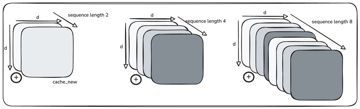
Original figureTop: standard attention decoding — each step reads O(ND) data twice from HBM (once each for the K and V caches) and writes two 1-D vectors; the KV Cache grows O(N) with the sequence. Bottom: linear attention — the state is a fixed D×D; per-step IO is independent of sequence length.
What's the price? Expressiveness. Clearest when you decompose attention into three steps:
Make the qk scores non-negative — softmax uses the exponential; linear attention uses ELU+1;
Normalize by the total score;
Take a weighted average of the values.
All three steps survive, but the "non-negativizing" function in step one went from exponential to ELU+1 — a lower-expressiveness approximation of the softmax kernel. The exponential can produce sharp, winner-take-all attention distributions (precise retrieval of a single token); ELU+1 produces flatter, blurrier distributions. The actual accuracy loss depends on architecture and task, but on tasks that require "fishing one precise detail out of a long context," naive linear attention's disadvantage is real.
THE CORE TENSION · MEMORY CAPACITY
A more fundamental problem hides inside the "fixed-size state": the KV Cache reserves an independent slot for every historical token (lossless but unbounded growth); the \(D \times D\) state compresses all history into a fixed matrix (bounded, but with inevitable mutual interference). It's like endlessly stuffing cards into a fixed-size drawer — the more you stuff, the more the writing on the cards blurs together. DeltaNet, next chapter, exists to answer "what do you do when the drawer is full."
TAKEAWAYS
Linear attention = replace softmax with a feature map, then use associativity to fold history into a fixed D×D state.
Gains: O(1) IO per decoding step, state independent of sequence length; costs: duller attention distributions, weaker precise retrieval.
It reconnected the Transformer to its RNN bloodline — and every linearization work since has been patching that bloodline's two defects: precision and memory management.
05DeltaNet: A Whiteboard That Corrects Itself
DELTA RULE · SCHLAG ET AL. 2021 · FAST WEIGHT PROGRAMMERS
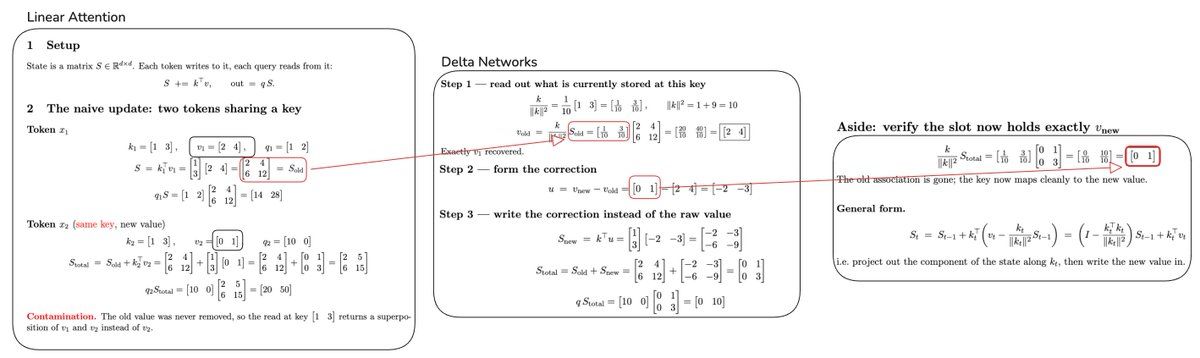
A finite-capacity cache inevitably faces overwriting and interference. In linear attention, token \(i-1\)'s state has no slot of its own — it got added into the same \(D \times D\) matrix. When a new query wants to read back some early token's independent representation with precision, it no longer can.
This "addition" is both the source of efficiency and the source of disaster: updating the cache by accumulation rather than concatenation is what keeps it from O(N) bloat; but accumulation is also what lets information pollute each other. Schlag et al. put it perfectly in Linear Transformers Are Secretly Fast Weight Programmers:
"When sequence length exceeds storage capacity, the model enters an 'over-capacity' regime. To function there, the model should learn to interact dynamically with memory contents, selectively deciding which key-value associations to keep and which to delete. A purely additive rule is unsuited for this purpose… endlessly adding new associations to a finite memory inevitably hits the limit."
Original figureA purely accumulative state matrix: new associations (green) pile onto old ones, nothing is ever deleted. Once capacity is exhausted, what you read out is an aliasing of all the history.
5.1 First, understand: an associative-memory whiteboard
Look at how a single association is stored and retrieved. Write \(S = k^\top v\) (outer product); read with the same key: \(k(k^\top v) = (kk^\top)v = \|k\|^2 v\). That is, the readout is exactly the value times the squared norm of the key — normalize k to unit length (or divide by the norm after reading) and you get v back losslessly.
Original figureThe outer product \(k^\top v\) forms an addressable associative memory: write with one key, read with the same key. Many associations with different keys can coexist in one matrix — as long as the keys are near-orthogonal, interference stays small; that is the geometric meaning of "capacity."
Q here is a learnable pointer: \(W_q\) and \(W_k\) read the same residual stream, and the query for a fact will point toward the key direction under which that fact was originally written. This machinery descends directly from last century's Hopfield networks — Transformer attention was always a modern associative memory.
5.2 The delta rule: erase first, then write
The delta rule (the modern incarnation of the Widrow-Hoff rule) updates like this:
First read the cache with the current key: \(v_{old} = k_i S\), see what's stored at this location now;
Compute the delta: the difference between the new value you want and the old value, scaled by write strength \(\beta\): \(u_i = \beta_i (v_i - v_{old})\);
Write the delta back: \(S \leftarrow S + k_i^\top u_i\).
defforward(self, x, mask=None, cache=None):
# x: (b, t, d)
b, t, d = x.shape
...
q = F.normalize(F.silu(q), dim=-1) # (b,h,t,dh), unit length
k = F.normalize(F.silu(k), dim=-1) # (b,h,t,dh), normalized: lossless readout
beta = torch.sigmoid(self.w_beta(x)).view(b, 1, t, 1) # (b,1,t,1), new: per-token write strength
S = cache if cache is not None else 0.0 # (b, h, dh, dh)
v_old = k @ S # (b,h,t,dh)×(b,h,dh,dh) → (b,h,t,dh), read old info at this key
u = beta * (v - v_old) # (b,h,t,dh), delta: write only what's truly new
S = S + k.transpose(-1, -2) @ u # (b,h,dh,t)×(b,h,t,dh) → (b,h,dh,dh), same outer-product write
o = q @ S # (b,h,t,dh)×(b,h,dh,dh) → (b,h,t,dh), readout (no normalizer needed)
o = o.transpose(1, 2).contiguous().view(b, t, d) # (b, t, d)return self.o_proj(o), S # (b,t,d); cache S: (b,h,dh,dh)
Old information is removed in a targeted way and new information is written in its place — the cache turns from an "append-only ledger" into an "editable whiteboard." \(\beta\) is input-dependent (a sigmoid gate): the model learns for itself how hard each token should rewrite memory.
WHY "FAST WEIGHT PROGRAMMERS"
In this view, the state matrix \(S\) is itself a "fast weight" network — ordinary weights update slowly via gradient descent (at training time), while \(S\) is programmed in real time by the input data during the forward pass (at inference time). DeltaNet lets the model learn to write its own program: precisely modify its own memory matrix based on current content. This is a modern revival of the 1990s Schmidhuber line of thought, and a member of the "in-context learning as implicit gradient descent" family of theories.
TAKEAWAYS
Linear attention's state is an associative memory; purely additive writes cause information aliasing beyond capacity.
Delta rule = read old value → compute difference → write back the delta: targeted modification instead of blind accumulation.
Write strength β is data-driven; the model learns "when to edit, and how hard" by itself.
06Parallelizing DeltaNet: The Chunking Trick
PARALLELIZING LINEAR TRANSFORMERS WITH THE DELTA RULE · YANG ET AL. 2024
FROM THE ORIGINAL AUTHOR
"This is the hardest section of the whole article — I spent about seven hours building a workable understanding, so I build the explanation from the implementation outward." We keep that route in this chapter: first see the problem clearly, then the mathematical reparameterization, then land on code. One-sentence summary: DeltaNet writes the transition matrix of a first-order linear recurrence as a product of generalized Householder transforms, enabling a chunk-parallel forward pass that makes linear-time training hardware-friendly.
6.1 The problem: sequential dependency at prefill
Token-by-token recurrence is natural at inference, but during training/prefill, if you run T tokens through the delta rule one at a time, the GPU just sits there watching:
S = torch.zeros(b, h, dh, dh) if cache is None else cache # (b,h,dh,dh)
outs = []
for i inrange(t): # purely sequential loop, T small matrix ops
k_i = k[:, :, i:i+1] # (b,h,1,dh)
v_i = v[:, :, i:i+1] # (b,h,1,dh)
b_i = beta[:, :, i:i+1] # (b,1,1,1), scalar write strength
v_old = k_i @ S # (b,h,1,dh)×(b,h,dh,dh) → (b,h,1,dh)
u_i = b_i * (v_i - v_old) # (b,h,1,dh)
S = S + k_i.transpose(-1, -2) @ u_i # (b,h,dh,1)×(b,h,1,dh) → (b,h,dh,dh), write
outs.append(q[:, :, i:i+1] @ S) # (b,h,1,dh)
o = torch.cat(outs, dim=2) # (b,h,t,dh)
Unlike standard attention: the delta rule must "read–correct" at every key, and step \(i\) depends on the state corrected at step \(i-1\). The path to parallel matrix multiplication is anything but obvious. In fact, even without the delta correction, naive linear-attention prefill is equally sequential (\(S\) accumulates step by step).
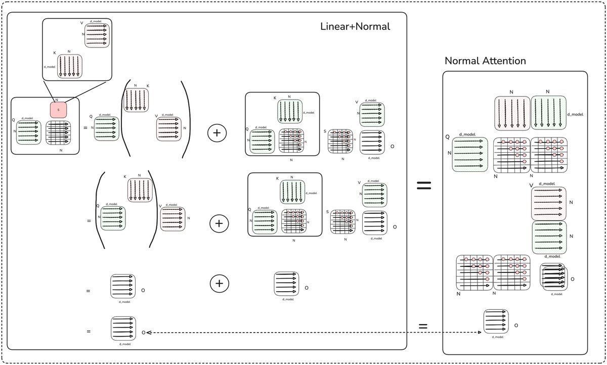
6.2 Chunking: stitching two orders of association
The way out is chunking. Cut the sequence into chunks of length C (in practice C is often 64 or 128, because tensor-core instructions are most efficient at that granularity, e.g. NVIDIA's UMMA):
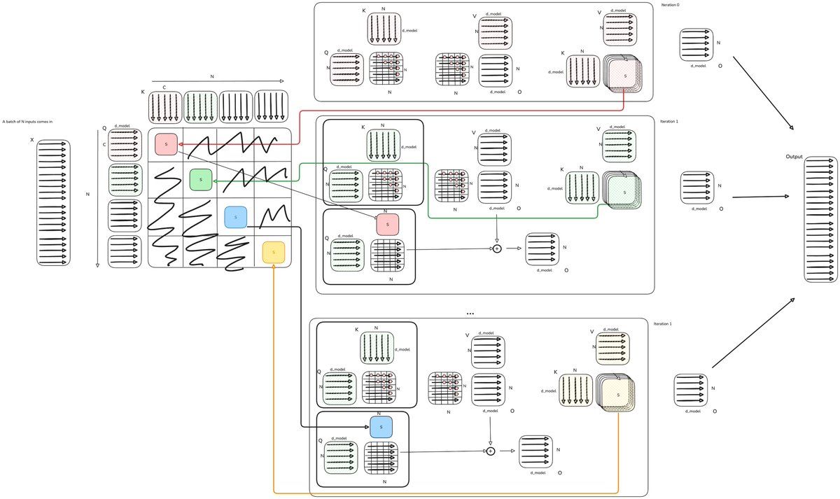
Inside a chunk: compute in the order \(q(k^\top v)\) — scores first, then masked weighting, i.e. "true attention" mode; intra-chunk complexity \(O(C^2)\);
Across chunks: go in the order \((k^\top v)q\) — at each chunk's end, fold the whole chunk's contribution into the state \(S\); the next chunk reads from the state with one matrix multiply, i.e. "recurrent" mode.
Original figureThe compute graph of chunked linear attention: the small squares on the diagonal are intra-chunk attention (score-first); everything else is stitched through the state S (state-first).Original figureThe intermediate tiles produced by each chunk are folded into the state S as the next chunk's "context summary."
S = torch.zeros(b, h, dh, dh) if cache is None else cache # (b,h,dh,dh)
outs = []
for i inrange(t // C): # only t/C iterations, each a big matmul
q_c = q[:, :, i*C:(i+1)*C] # (b,h,C,dh)
k_c = k[:, :, i*C:(i+1)*C] # (b,h,C,dh)
v_c = v[:, :, i*C:(i+1)*C] # (b,h,C,dh)
o_prev = q_c @ S # (b,h,C,dh)×(b,h,dh,dh) → (b,h,C,dh), all history before this chunk
attn = (q_c @ k_c.transpose(-1,-2)).tril() # (b,h,C,C), masked intra-chunk attention
o_curr = attn @ v_c # (b,h,C,C)×(b,h,C,dh) → (b,h,C,dh)
o = o_prev + o_curr # (b,h,C,dh)
S_new = k_c.transpose(-1,-2) @ v_c # (b,h,dh,C)×(b,h,C,dh) → (b,h,dh,dh), fold the chunk into the state
S = S + S_new # (b,h,dh,dh)
outs.append(o)
o = torch.cat(outs, dim=2) # (b,h,t,dh)
The cost decomposition is elegant: a fixed part \(2Ld^2\) (state maintenance, independent of C) + a growing part \(2LCd\) (the score matrices on the diagonal). C = L degenerates to standard attention (the second term becomes \(2L^2d\), quadratic); C = 1 is pure linear attention. Intermediate C trades a little intra-chunk compute for hardware utilization — C=1 is cheapest in pure FLOPs, but not in wall-clock time: GPUs only run fast when work maps to large matrix multiplies.
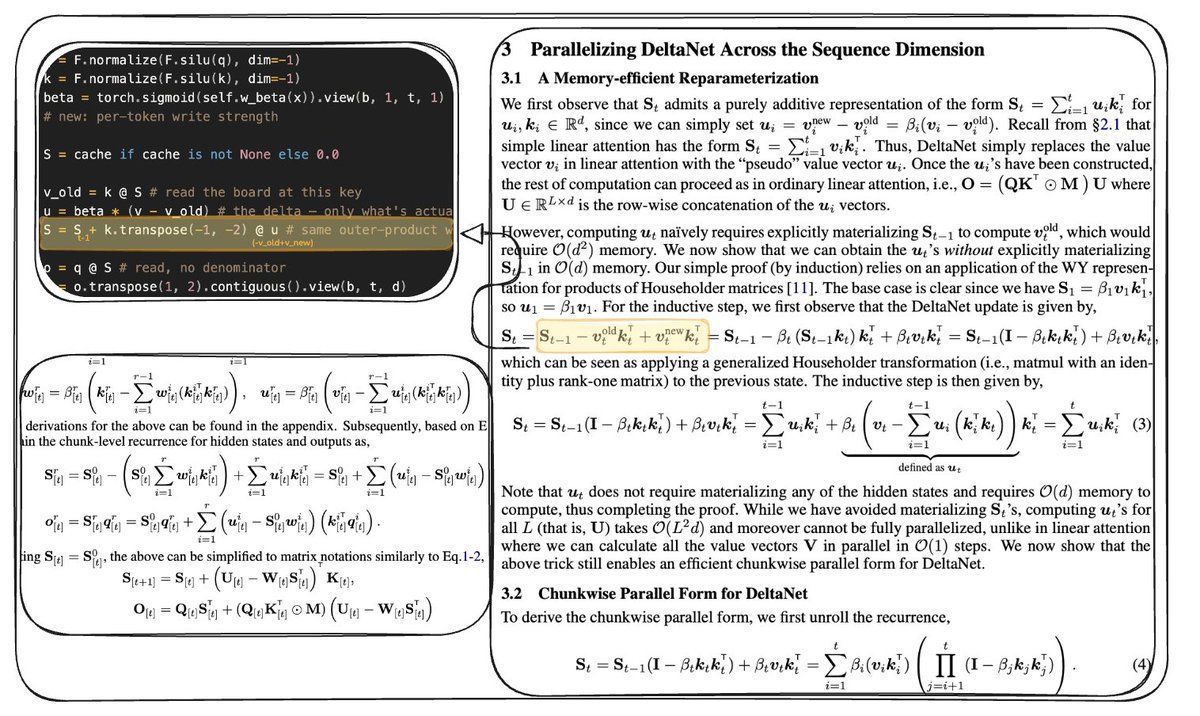
6.3 Squeezing the delta correction into chunks: WY reparameterization
Applying the same chunking idea directly to the delta rule hits a wall: each key's correction depends on the state at that moment, while chunk-parallelism requires all corrections within a chunk to be computed at once:
v_old = k_i @ S               # (…,1,dh)×(…,dh,dh) → (…,1,dh)
u_i = b_i * (v_i - v_old)     # (…,1,dh), every u_i depends on S after all prior corrections
We would have to pass through every intermediate state in order to know what to subtract — without mathematical reparameterization, no parallelism. The authors' approach: expand the recurrence
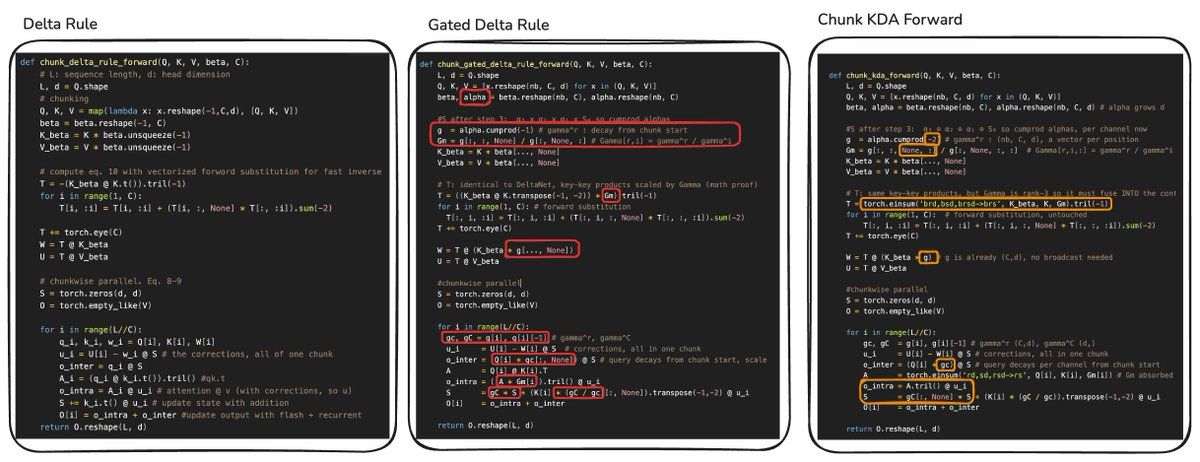
and discover that \(S_T\) can be written as the initial state left-multiplied by a string of \((I - \beta k k^\top)\) products, plus a weighted sum of \(v k^\top\) terms — exactly the WY representation (the compact form of products of Householder transforms in numerical linear algebra). The corrections \(u\) can be solved all at once by forward substitution on a C×C lower-triangular matrix. The full four-step derivation from recurrence to expansion is in Appendix B; here we land directly on the code — the chunked code computes all C deltas of a chunk at once:
defchunk_delta_rule_forward(Q, K, V, beta, C):
# Q,K,V: (L, d); beta: (L,); C: chunk length
L, d = Q.shape
# chunk
Q, K, V = map(lambda x: x.reshape(-1, C, d), [Q, K, V]) # each (L/C, C, d)
beta = beta.reshape(-1, C) # (L/C, C)
K_beta = K * beta.unsqueeze(-1) # (L/C, C, d)
V_beta = V * beta.unsqueeze(-1) # (L/C, C, d)# vectorized forward substitution: invert (I + strictly lower triangular)
T = -(K_beta @ K.t()).tril(-1) # (L/C, C, C), strictly lower triangularfor i inrange(1, C):
T[i, :i] = T[i, :i] + (T[i, :, None] * T[:, :i]).sum(-2)
T += torch.eye(C) # (L/C, C, C), lower triangular, unit diagonal
W = T @ K_beta # (L/C,C,C)×(L/C,C,d) → (L/C, C, d), corrected keys
U = T @ V_beta # (L/C, C, d), corrected values (all deltas included)# chunk-parallel main loop
S = torch.zeros(d, d) # (d, d)
O = torch.empty_like(V) # (L/C, C, d)for i inrange(L // C):
q_i, k_i, w_i = Q[i], K[i], W[i] # each (C, d)
u_i = U[i] - w_i @ S # (C,d) − (C,d)×(d,d) → (C, d), the chunk's corrections at once
o_inter = q_i @ S # (C, d), history contribution (recurrent mode)
A_i = (q_i @ k_i.t()).tril() # (C, C), intra-chunk attention scores
o_intra = A_i @ u_i # (C,C)×(C,d) → (C, d), intra-chunk contribution (attention mode)
S += k_i.t() @ u_i # (d,C)×(C,d) → (d, d), update the state
O[i] = o_intra + o_inter # (C, d)return O.reshape(L, d) # (L, d)
Original figureChunk-parallel delta rule: the C×C intra-chunk dependencies are solved at once by inverting a lower-triangular matrix; across chunks, the state is still passed along.
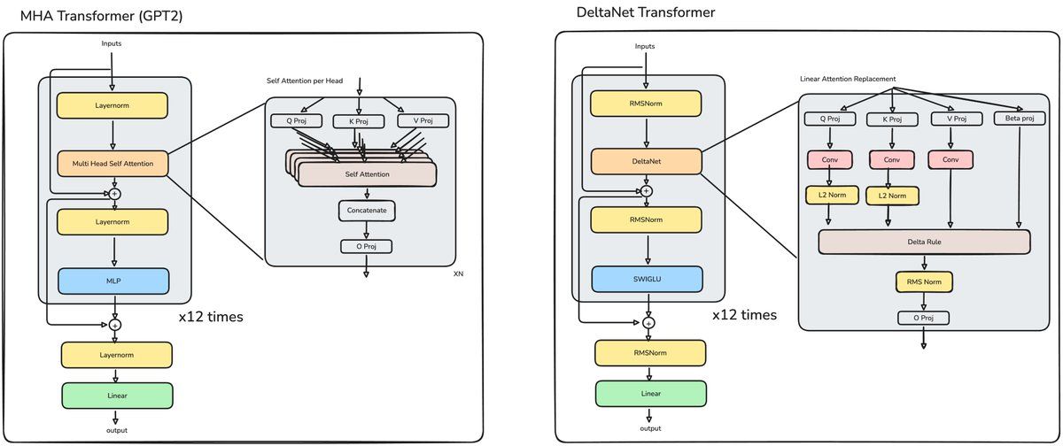
With this we reach the first milestone comparison — the standard multi-head attention Transformer vs the DeltaNet Transformer:
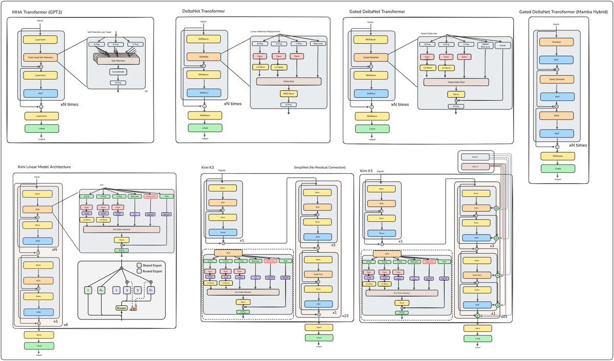
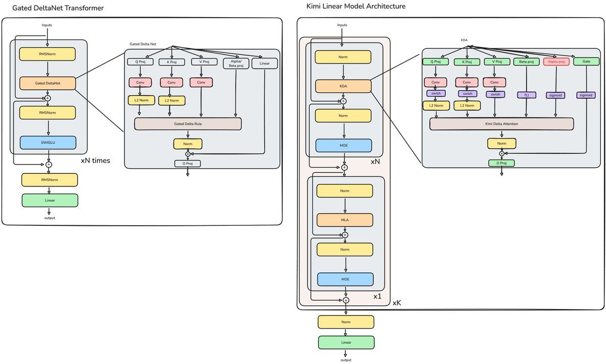
Original figureMHA (left) vs the DeltaNet Transformer (right): nearly isomorphic — same QKV projections, output projection, residual stream; only the core memory mechanism differs: one maintains an ever-growing KV cache with softmax retrieval, the other a fixed-size, precisely editable state matrix.
TAKEAWAYS
Chunking = intra-chunk attention (exact, quadratic) + inter-chunk recurrence (compressed, linear); C is the knob between precision and efficiency.
WY reparameterization turns "correct one by one" into "solve the whole chunk at once," letting the delta rule saturate tensor cores.
Note the recurring theme of this article: mathematically equivalent transformations in exchange for hardware friendliness — same spirit as FlashAttention.
Half of the Gated DeltaNet in the next chapter descends from Mamba. So before the "forget gate," we must meet linear attention's parallel universe — State Space Models (SSM).
7.1 From control theory to deep learning: the math of SSMs
The state space model is an antique of control theory: a continuous-time linear time-invariant system
where \(x(t)\) is the input signal (in an LLM, one dimension of a token embedding), \(h(t) \in \mathbb{R}^N\) is the hidden state, \(A\) the state-transition matrix, \(B\) and \(C\) the input/output projections. To handle discrete token sequences, discretize with Zero-Order Hold:
The discretized recurrence is a linear RNN — per-step cost independent of sequence position, which is how SSMs achieve \(O(L)\) total complexity (instead of \(O(L^2)\)). Its resemblance to linear attention's \(S_t = S_{t-1} + k_t^\top v_t\) is no coincidence: both compress all of history into a fixed-size hidden state — they just speak different dialects.
Key milestones of the SSM family:
S4 (Gu et al., 2021): the first SSM to beat Transformers on very long sequences. The core: initialize \(A\) with the HiPPO matrix (a mathematically optimal "history compression basis") and train in parallel via diagonalization + convolution tricks. But S4's transition matrix is fixed — it doesn't change with input, like a memory machine that can't adjust to content.
Mamba (Gu & Dao, 2023): make \(B\), \(C\), and the discretization step \(\Delta\) all functions of the input — "selective." The model can decide per content whether to remember carefully or ignore this step. The cost: the convolutional parallel form is lost, so a hardware-aware parallel scan algorithm was invented to run the recurrence in SRAM. Mamba was the first linear-time architecture to match same-size Transformers on language modeling.
Mamba-2 / SSD (2024): revealed the strict duality between SSMs and linear attention — a scalar-gated SSM is "linear attention with a forget gate." This insight unified the two parallel universes and paved the road directly to Gated DeltaNet (next chapter).
Mamba's selection mechanism: make parameters content-dependentSELECTIVE SCAN
Classic SSM parameters \(A, B, C, \Delta\) are time-invariant — the same for every token, unable to decide what to remember or ignore based on content. Mamba makes \(B, C, \Delta\) input-dependent:
where \(s_B, s_C, s_\Delta\) are learnable linear projections. The effect: large \(\Delta_t\) → attend more to current input ("forget" history); small \(\Delta_t\) → rely more on historical state. But with parameters input-dependent, the recurrence is no longer time-invariant and can't parallelize via convolution — hence Mamba's dedicated hardware-aware selective scan algorithm.
The SSD duality: two parallel universes are the same thingSTATE SPACE DUALITY
Expand the SSM recurrence into "convolutional form":
Compare with linear attention's expansion \(o_t = \sum_s \phi(q_t)\, \phi(k_s)\, v_s\) — \(\bar{A}^{t-s}\) plays exactly the role of an "attention score that decays with distance." Mamba-2 exploited this duality to design structured matrix multiplication (SSD), letting SSMs be implemented efficiently with chunked matmuls like attention. This duality is the key to Chapter 08: the SSM decay gate and DeltaNet's precise writing can merge within one mathematical framework.
Figure 7-1 (self-drawn): two parallel universes. SSMs maintain a vector state with per-channel decay; linear attention maintains a matrix state with key-outer-product writes. Mamba-2 proved they share the same root.
7.2 Other runners on the same track
Architecture
Year
Core idea
One-line verdict
RWKV
2023
Reformulates an RNN into parallel-trainable form: token-shift + exponentially decayed "softmax-free attention"
Open-source community darling; proved RNNs can train to 14B scale
RetNet
2023
Microsoft's retention mechanism: three equivalent forms — parallel training / recurrent inference / chunkwise recurrent
Highly isomorphic to linear attention
Hyena
2023
Replaces attention with ultra-long convolutions + data-controlled gating
Flagship of the long-convolution route, later absorbed into SSMs
S4 / S4D
2021+
HiPPO initialization + diagonalized SSM
Theoretical founder; engineering baton passed to Mamba
Mamba / Mamba-2
2023/24
Input-dependent selection + hardware-aware scan; the SSD duality
The LSTM inventors' "revenge"; philosophically kin to DeltaNet
HISTORY'S SENSE OF HUMOR
In the 1990s, the RNN (LSTM) was dethroned by the Transformer; in the 2020s, researchers queued up to bring the RNN back — just to kill the Transformer's \(O(N^2)\) and KV Cache. But watch how it ends: the winner is not any "purebred" architecture, but a hybrid — starting next chapter you'll see that every frontier model is a blend of "linear recurrent memory + periodic full attention."
08Gated DeltaNet: Learning to Forget
GATED DELTA NETWORKS · YANG ET AL. 2024
Back to the main thread. DeltaNet gave us the ability to precisely edit the cache: every arriving key carrying a new fact can read the old content at its location and replace it in a targeted way. But it has a blind spot —
It can only forget "associations that have a replacement." Want to clear a batch of old memories when the topic changes? Want unimportant facts to decay over time to make room? The delta rule can't: its eraser wipes only the small patch under one key at a time.
Conversely, if we were doing purely additive linear attention, adding "forgetting" is actually easy — it takes only a single scalar parameter:
S_old = cache # (b,h,dh,dh)
S_new = k @ v # (b,h,dh,t)×(b,h,t,dh) → (b,h,dh,dh)# cache = S_old + S_new # the old pure accumulation
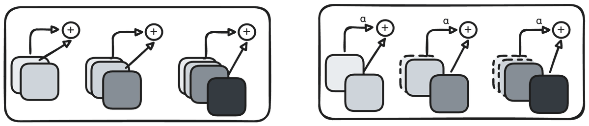
cache = alpha * S_old + S_new # alpha: (b,1,t,1) scalar gate → (b,h,dh,dh), decay old state, then write at full strength
Original figureThe forget gate α: each step first decays the whole state matrix proportionally, then writes the new association. The state no longer grows without bound.
This is exactly Mamba-2's contribution: decay the old cache first, then write the new content at full strength, preventing unbounded state inflation. But uniform decay has an obvious flaw — it doesn't distinguish how important associations are. To forget one specific association, every association must age by the same proportion. The delta rule is the exact opposite: it can update a single fact surgically, but can't batch-decay the rest.
Gated delta rule = Mamba's gating × the delta rule's precision. Introduce the parameter \(\alpha_t\): at \(\alpha = 1\) it degenerates to the pure delta rule; at \(\alpha = 0\) it wipes memory clean. The update:
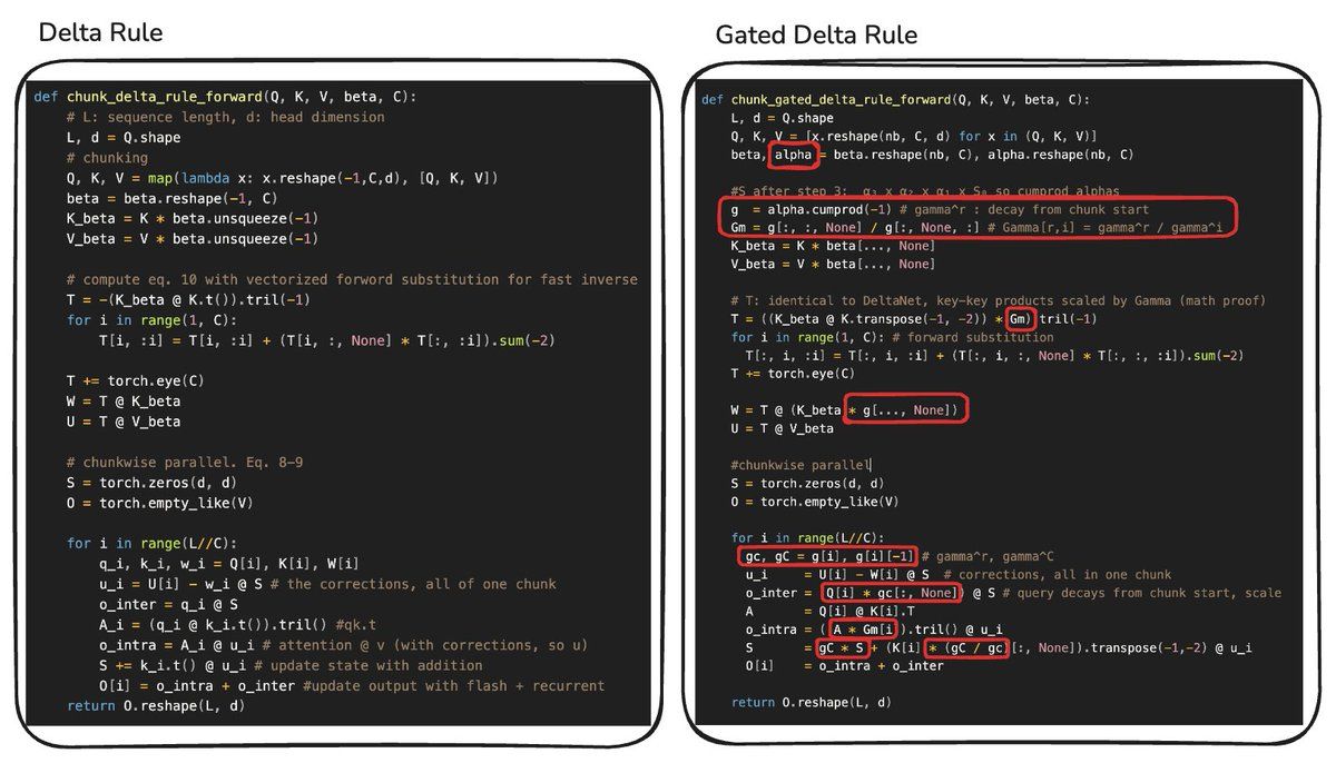
The implementation reuses Chapter 06's WY reparameterization; the math barely changes — just one more data-dependent scalar between 0 and 1 controlling the decay of the previous state. The difficulty is again engineering: the chunk-parallel form must handle cumulative decay —
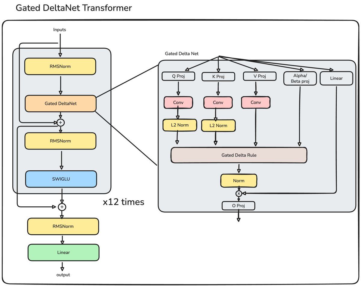
Original figureGated DeltaNet's chunked code. Note the γʳ/γⁱ terms in the formulas: a token written at time x, when read at time x+t, has already been multiplied by αₓ·αₓ₊₁·…·αₓ₊ₜ — a "prefix product," the multiplicative-world counterpart of the prefix sum, which likewise needs discretization tricks to parallelize.Original figureGated DeltaNet's final form: k/v/β/α are all produced by input projections — the model decides per content "how much to decay, how hard to write, what to write."
CONCEPT DISTILLATION · THE THREE OPERATIONS OF MEMORY MANAGEMENT
At this point, the linearized model has assembled the complete operation set of memory management: write (outer-product accumulation, linear attention) → edit in place (delta rule) → global decay (gating). These map neatly onto human memory's "remember, correct, fade." One last puzzle piece is missing — finer-grained forgetting — and that's KDA's business in the next chapter.
TAKEAWAYS
The delta rule can correct but not fade; Mamba can fade but not correct — Gated DeltaNet does both.
α and β are both data-driven: the model decides its memory policy in real time, in context.
Cumulative decay = the multiplicative prefix sum, and the main engineering obstacle to chunk-parallelization.
09KDA and Kimi Linear
KIMI DELTA ATTENTION · KIMI LINEAR · 2025
At this stage, researchers began trying hybrid architectures — interleaving multiple attention forms in one model, e.g. mixing Gated DeltaNet with Mamba, or linear layers with full-attention layers. In 2025, Kimi Linear pushed this path to a landmark conclusion:
KIMI LINEAR'S CORE CLAIM
Under strictly controlled comparison (same data, same compute), Kimi Linear beats the full-attention baseline across the board — not "matches," surpasses — while improving decoding throughput by up to 6× and reducing KV Cache by up to 75%. It positions itself as a "drop-in architectural replacement," not a long-sequence-only patch.
9.1 KDA: fine-grained gating
Kimi Delta Attention's (KDA) key improvement over Gated DeltaNet is upgrading the forgetting from a scalar to a per-channel vector: no longer decaying the entire state matrix with a single α, but learning an independent decay rate for every feature channel.
Original figureScalar gating vs fine-grained gating: GDN's α is one scalar per head (the whole memory block lives and dies together); KDA's α is a per-channel vector (every dimension of memory has its own half-life) — important channels decay slowly, noisy channels decay fast.
The update rule's skeleton is unchanged, but the code gains one reshape:
Original figureKDA's chunked implementation. Note the line alpha.reshape(nb, C, d) — it carries the paper's most important contribution: per-channel fine control over memory decay.
Fine-grained gating is not simply "adding parameters." It has a precise mathematical function: installing a tiered recycling system on a capacity-limited memory — an independent decay rate per channel is equivalent to soft memory-partition management in feature space. This is exactly the engineering solution to Chapter 05's "over-capacity aliasing" problem.
9.2 Kimi Linear's complete recipe
Side by side with the DeltaNet Transformer, Kimi Linear introduces three major changes:
Hybrid architecture: MLA (Multi-head Latent Attention) layers interleaved in — 3 KDA layers per 1 full-attention layer;
MoE replaces the MLP: feed-forward networks swapped for mixture-of-experts layers;
Expanded α projection: extra capacity for the DeltaNet mechanism via the alpha projection (the fine-grained gating above).
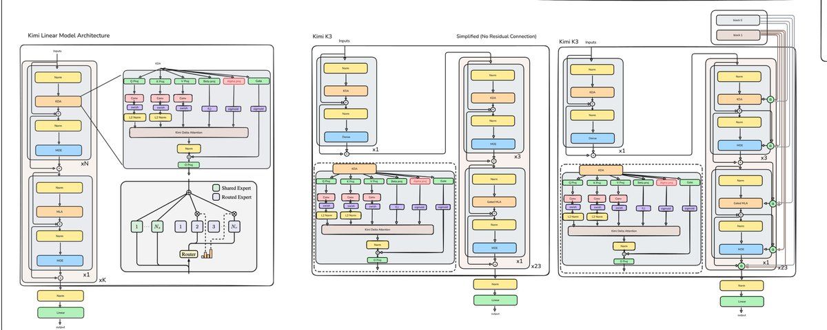
Original figureKimi Linear (right) vs the DeltaNet Transformer (left): KDA layers carry most of the sequence modeling; periodically appearing MLA layers provide lossless softmax-precise retrieval; all MLPs become MoE.
Details of MLA and MoE are deferred to Chapter 10. Here, stress one important argument of the original: this is not blind ingredient-stacking. Every added capacity serves a concrete mathematical purpose — per-channel α gives fine control over memory decay; periodic MLA restores the precise retrieval that linear states necessarily lose; MoE adds knowledge capacity without adding per-token compute.
Scaling laws still hold, but capacity must be added in the right places, in forms the system can digest. Every architecture on this evolutionary line is targeted capacity expansion for a specific defect of the previous system.
TAKEAWAYS
KDA = Gated DeltaNet + per-channel forget gates; every dimension of memory gets its own half-life.
Kimi Linear = 3:1 hybrid KDA/MLA + MoE; beats full attention under controlled comparison, with 6× faster decoding.
"Hybrid" becomes the theme: linear recurrence for efficiency, periodic attention for fidelity.
10Interlude III: MoE and MLA in Depth
MIXTURE-OF-EXPERTS · MULTI-HEAD LATENT ATTENTION (NEW BACKGROUND CHAPTER)
The two pillars of Kimi Linear and Kimi K3 — MoE and MLA — got only passing mention in the original. But they were the main battleground of the 2024–2026 LLM arms race (DeepSeek's rise rests almost entirely on these two), and each deserves a section.
10.1 MoE: the art of sparsity
Recall Chapter 02's parameter breakdown: in GPT-2, about two-thirds of the parameters live in the MLP. The MLP is considered the model's "knowledge warehouse" (attention routes information; the MLP stores facts). So here's a tempting idea: make many copies of the MLP, but let each token use only a few of them — parameter count (knowledge capacity) explodes while per-token compute barely changes. That is Mixture-of-Experts.
Figure 10-1 (self-drawn): the MoE forward pass. The router scores every expert for each token; only the Top-K (K=2 here) experts are activated, and outputs are weighted by gate values. Dashed experts are not computed this step.
Key design points and history:
Origins: Shazeer et al.'s Sparsely-Gated MoE in 2017 (the LSTM era!); in 2021 Google's Switch Transformer (simplified to Top-1 routing) and GShard took MoE to ten-thousand-GPU scale.
Load balancing: routers tend to "despise the poor" — a few experts get picked frantically while the rest starve, and training collapses. The classic fix is an auxiliary load-balancing loss forcing uniformity, but it hurts model quality; DeepSeek-V3 pioneered the auxiliary-loss-free route: give each expert a dynamic bias term that affects only routing decisions and never enters gradients — balance and quality at once.
Fine-grained + shared experts (DeepSeekMoE, 2024): cut experts smaller and more numerous (greater combinatorial flexibility), and designate a few shared experts that handle common knowledge for all tokens while routed experts learn only specialized knowledge — mitigating knowledge redundancy. Kimi K3's 898 experts (2 shared + 896 routed) is the jumbo version of this idea.
The open-source detonation: Mixtral 8×7B (2023) proved even a mid-size MoE can crush same-tier dense models; after that, DeepSeek-V3 (671B / 37B activated), Qwen3-MoE, and Kimi K2 (1T / 32B activated) made MoE the default form of frontier models.
The cost: memory must hold all experts (parameters don't shrink), training communication is complex (expert-parallel AllToAll), and expert utilization is poor at small inference batches. What MoE saves is FLOPs, not memory.
10.2 MLA: distilling the KV Cache
§3.1 said MLA is the newest weapon in the siege on KV Cache; now let's take it apart. GQA's idea is "let Q heads share K/V"; MLA (DeepSeek-V2, 2024) is more radical: jointly low-rank-compress all heads' K and V into a single latent vector \(c_t\), and cache only that, decompressing into each head's K/V on use.
Standard MHA: \(K = XW_K,\ V = XW_V\), requiring full K and V in cache. MLA introduces a low-dimensional latent:
\[ c_t^{KV} = W^{DKV}\, h_t \;\in\; \mathbb{R}^{d_c} \qquad\text{(only this and the RoPE part are cached)} \]
\[ k_t = W^{UK}\, c_t^{KV}, \qquad v_t = W^{UV}\, c_t^{KV} \]
Typical configuration: \(d_c = 512\), while standard MHA's per-token KV cache dimension might be \(64 \times 128 = 8192\) — ~16× compression.
Matrix absorption is the most elegant step: the decompression matrix \(W^{UK}\) can be pre-multiplied into the query projection before inference, and \(W^{UV}\) into the output projection — at inference you never actually decompress K/V at all; attention is computed directly in the compressed space.
Decoupled RoPE: RoPE's rotation is fundamentally at odds with "content compression" (a rotated vector can't be low-rank factored), so MLA splits position information into a small set of dedicated dimensions (e.g. 64) that get RoPE applied separately; this small piece \(k^R\) is cached alongside, while the main compressed body stays a pure content representation.
Figure 10-2 (self-drawn): MLA's compress–decompress structure. The cache holds only one low-dimensional latent vector (512 dims + a 64-dim RoPE component in DeepSeek-V2) — over 90% smaller than MHA.
Adding multi-head latent attention's exploitation of "redundancy between heads," MLA achieves an anomalous result: a cache far smaller than GQA's, with quality better than MHA's.
WHY MLA + LINEAR ATTENTION IS A MATCH MADE IN HEAVEN
Back to Kimi Linear's 3:1 hybrid: KDA layers have fixed state and produce no KV Cache at all; the few MLA layers produce a tiny cache — the whole model's long-context inference cost is squeezed extremely low. That is why "linearization + MLA" became the golden combination of 2025–2026 hybrid architectures. Chapter 11's Gated MLA evolves it one step further.
TAKEAWAYS
MoE: routing decouples "parameter count" from "compute" — knowledge without FLOPs; the core difficulty is load balancing.
MoE saves training/inference compute; MLA saves inference memory bandwidth — each strikes one of the two legs of LLM cost.
11Kimi K3: The 22,580× Endpoint (For Now)
KIMI K3 · 2026 · 2.8T-PARAMETER HYBRID ARCHITECTURE
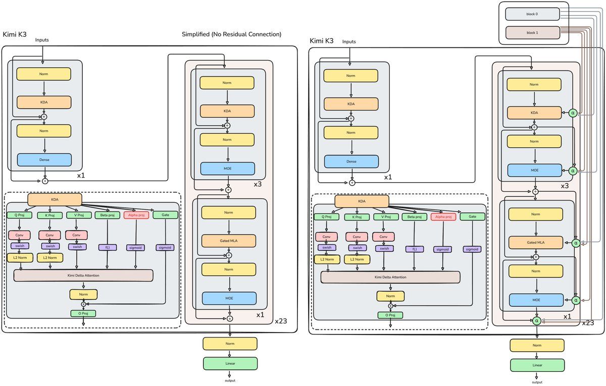
All the threads converge here. Kimi K3's language backbone is a scaled-up Kimi Linear: 23 four-layer macrocycles — within each macrocycle, 3 layers use Kimi Delta Attention and the 4th uses MLA; the first layer uses a dense feed-forward network, everything else becomes latent-space MoE.
Compared with Kimi Linear, the change list looks unremarkable at first:
Substantially larger scale (to 2.8T parameters)
Blockwise AttnRes every 12 layers (detailed in Chapter 12)
Query LoRA and output gating for MLA
Latent-space MoE
The SiTU activation function
Gated MLA
The division of labor is the same as ever: KDA provides constant-state recurrent memory, while periodic MLA layers preserve full softmax retrieval over the context. One diagram to rule the whole model:
Original figureSimplified Kimi K3 architecture: the 23 × (3×KDA + 1×MLA) macrocycle structure, assisted by AttnRes, Gated MLA, latent-space MoE, and SiTU.
11.1 Three direct changes: Gated MLA, latent-space MoE, SiTU
Gated MLA: decides how much of what MLA retrieves may enter the residual stream — a gate projected from the input, multiplied element-wise with the attention output. In essence it puts a faucet on the "precise retrieval channel": retrieval is accurate, but how much of it to let into the trunk is decided by context.
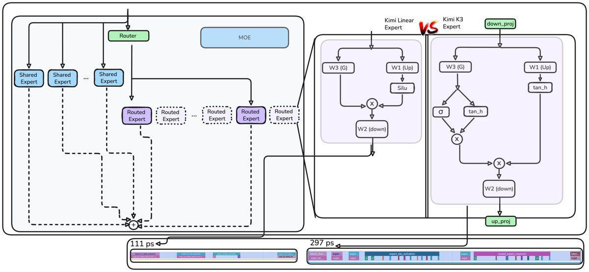
Latent-space MoE: in a traditional MoE, the router sends each token to several experts by dot-product similarity. Kimi K3 has 898 experts: 2 shared experts process every token, and the router picks 16 of the remaining 896 for each token. K3's further innovation is letting experts work in a compressed latent space:
Original figureLatent-space MoE: the input is first down-projected into the shared experts' compressed space; experts run their forward there, and the sum is up-projected back to full dimension at the end. Expert forward FLOPs are nearly halved.
The SiTU activation: K3 also replaces the activation inside experts. Instead of the old "expand → SiLU → element-wise gate multiply → contract" route, it uses SiTU:
d = x.shape[-1] // 2 # x: (..., 2d), first half gate, second half up
gate = x[..., :d].to(torch.float32) # (..., d)
up = x[..., d:].to(torch.float32) # (..., d)
situ_a = self.beta * torch.tanh(gate / self.beta) * torch.sigmoid(gate) # (..., d)if self.linear_beta is not None:
up = self.linear_beta * torch.tanh(up / self.linear_beta) # (..., d)return (situ_a * up).to(x.dtype) # (..., d)
Note the learnable \(\beta\) inside the tanh term: the saturation region of the gate becomes learnable — the model can tune the "hardness" of the activation per layer.
ENGINEERING REALITY · WHY FUSED KERNELS MATTER
This exposes a recurring inference-side difficulty: without a fused kernel, the new activation runs nearly 3× slower than the original path — what's free mathematically is all reads and writes in the memory hierarchy. One hedging optimization is experts working in the compressed latent space: much faster forward, FLOPs nearly halved. Architecture innovation must land together with kernel engineering — an industry truth the original author (an inference engineer at Baseten) repeatedly hints at.
The remaining changes: query LoRA, output gating, AttnRes
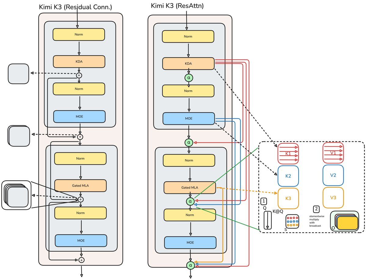
MLA gets LoRA low-rank adaptation on the query side and gating on the output, plus Blockwise Attention Residuals every 12 layers. AttnRes adds only ~2% inference latency, in exchange for two important gains: selective retrieval of early representations (mitigating residual dilution and hidden-state magnitude growth), and a 1.25× compute advantage (stronger at equal compute).
The last point is worth pausing on: AttnRes and MLA attack the same underlying limitation from different directions. KDA layers have constant state and necessarily discard information; MLA backstops with lossless retrieval along the sequence dimension (token context), while AttnRes backstops with selective retrieval along the depth dimension (representations of early layers). One patches horizontal memory, the other vertical memory.
11.2 The ledger: how 1T becomes 2.8T
In Chapter 02 we audited GPT-2's 124M; now we apply the same method to K3. First answer a common confusion: K3 doesn't have several times more layers than K2 — how did parameters grow from 1T to 2.8T? The answer hides in a three-factor MoE product:
\[
\text{MoE dominant parameters} \;=\; \text{MoE layers} \times \text{experts per layer} \times \text{params per expert}
\]
Item
Kimi K2
Kimi K3
Effect on total params
Total layers
61 (1 dense)
93 (1 dense)
Actual MoE layers 60 → 92, ~1.53×
Routed experts / layer
384
896
~2.33×
Expert input dim
7168
LatentMoE dim 3584
K3's per-expert input is narrower
Expert intermediate dim
2048
3072
K3's intermediate is wider
Selected per token
8 / 384 + 1 shared
16 / 896 + 2 shared
Affects activated compute, not total params directly
Official total / activated
1T / 32B
2.8T / 104B
Total params and per-token path are two different metrics
K2: first price out one SwiGLU expert60 × 384 EXPERTS
Per expert (gate, up, down matrices): \(P_{expert,K2} \approx 3 \times 7{,}168 \times 2{,}048 = 44{,}040{,}192 \approx 44.04\text{M}\)
Adding shared experts, KDA/MLA projections, embeddings, the dense layer, the vision encoder, etc., the official total is 2.8T.
Three-factor check: \((92/60) \times (896/384) \times (33.03/44.04) \approx 1.533 \times 2.333 \times 0.750 \approx 2.68\). So the answer is not "more layers" but MoE layers × expert density × per-expert size moving together — each expert shrank 25%, but the grid's expansion far outweighed it. (Note: this is a dominant-term approximation from public dimensions; actual checkpoints involve implementation details and accounting conventions.)
Every change answers a specific defect: retrieval precision, memory granularity, compute efficiency, numerical stability.
12AttnRes: Attention Across Depth
BLOCK ATTENTION RESIDUALS · REINVENTING THE RESIDUAL CONNECTION
(The original credits @chloey3k for help with this section.) In every forward pass, the input traverses a stack of layers — each layer an attention block (KDA or MLA) plus an MLP/MoE block. Traditionally, each layer's input is the equal-weighted sum of the original embedding and all previous layers' outputs:
\[ h_l = h_1 + \sum_{i=1}^{l-1} f_i(h_i) \]
where \(h_i\) is layer \(i\)'s input, \(h_1\) is the current token's embedding, and \(f_i(h_i)\) is layer \(i\)'s output. The problem: no selectivity. Different kinds of layers receive the same "hodgepodge" state even if they want to weight history differently; and because the recurrence is purely additive, later layers must learn ever-larger outputs to influence the accumulated residual — causing both "residual dilution" (early information drowned out) and continuously growing hidden-state magnitudes, which destabilizes training.
AttnRes's approach: stop treating everything equally — multiply each term of the sum by a dedicated weight:
Each weight \(\alpha_i\) is computed from a query-key dot product: queries are learned per layer, keys and values come from earlier residual-stream states; scores are normalized to sum to 1, then combined. The model no longer has to condition only on the immediately preceding layer — every layer can use its learned query to retrieve, from the entire depth history, the representations most useful to its current computation. This generalizes "attention" from the sequence dimension (between tokens) to the depth dimension (between layers).
Original figureAttnRes: at a block boundary, the current representation acts as query, scoring all historical block representations (softmax-normalized), then the weighted blend feeds the next stage. The residual stream changes from "add without choosing" to "a retrievable memory."
Applied at block granularity: a "block" is the element-wise accumulation of attention and MLP outputs over 12 decoder layers, stored as a single depth representation for later AttnRes mixing. Doing residual attention at every layer is too expensive; doing it only at fixed block boundaries captures most of the benefit at small cost — in K3, boundaries are 12 layers apart, and the 23 four-layer macrocycles yield 8 AttnRes blocks, which also improves inference speed.
The following is probably the most important part of the block_attn_res function:
V = torch.stack(blocks + [partial_block]) # [N+1, B, T, D] all historical blocks
K = norm(V) # [N+1, B, T, D], normalized for scoring
logits = torch.einsum('d, n b t d -> n b t', proj.weight.squeeze(), K) # [N+1, B, T], one score per block
h = torch.einsum('n b t, n b t d -> b t d', logits.softmax(0), V) # softmax over the block dim → weighted sum (B, T, D)return h # (B, T, D)
Four lines: stack all historical blocks → normalize and score with a learned vector → softmax over the "block" dimension → weighted mix. Note the softmax runs along dim 0 (the block dimension) — the competitors are not tokens, but depths.
CONCEPT DISTILLATION · ATTENTION'S THREE MIGRATIONS
Looking back over the whole article, the attention mechanism migrated three times: ① between tokens (2017, standard attention); ② between memory state and queries (2020+, linear attention/DeltaNet, where attention degenerates into state read/write); ③ between layers (2026, AttnRes). The same "query–match–weight" primitive has flowered in three dimensions: sequence, memory, and depth.
TAKEAWAYS
The residual stream's purely additive recurrence causes dilution and magnitude inflation; AttnRes gives each layer retrieval over depth history.
Block granularity (once per 12 layers) is the cost-benefit sweet spot: ~2% latency for 1.25× effective compute.
MLA backstops precise retrieval along sequence; AttnRes backstops it along depth — together they cover KDA's information loss.
Architecture is only half the story. What truly carried LLMs from the lab to a billion users over the past seven years is a set of methods that don't change the model's shape but bend the cost curve and the capability ceiling. We organize them along three lines: training, inference, and alignment.
13.1 Training: spend every watt where it counts
Scaling laws and Chinchilla (2020–2022)
OpenAI's 2020 scaling-law paper showed loss falls as a smooth power law in parameters, data, and compute — capability became predictable, giving the industry the confidence to burn money. But DeepMind's 2022 Chinchilla corrected a widespread mistake: models until then were generally "too big, underfed"; the optimal recipe is ~20 tokens per parameter. The 70B Chinchilla crushed the 280B Gopher. The Llama era then swung to "overfeeding" (small models eating trillions of tokens), because inference cost is the long-term dominant expense. This line of thinking persists today: set the inference budget first, then back out the training recipe.
Optimizers: Adam → Muon
AdamW ruled for eight years. In 2024, Keller Jordan's Muon (built for the NanoGPT speedrun) — with its idea of "Newton–Schulz orthogonalized updates for hidden-layer weight matrices" — improved sample efficiency ~2× on multiple benchmarks; Moonshot scaled it to large-model training (Kimi K2 uses MuonClip with QK-clip), bringing Muon into the frontline arsenal. Embeddings and output heads still use Adam — hybrid optimizers are the new normal.
Numerical precision and systems
BF16 mixed precision (2020+): the training standard; FP16's overflow troubles cured by BF16's large dynamic range.
FP8 training (DeepSeek-V3, 2024): first validation of FP8 mixed precision at very large scale, with per-block scaling — another cut to training cost.
Parallelism strategies: the combinatorics of data/tensor/pipeline/expert/sequence parallelism (Megatron, ZeRO, FSDP) — effective compute utilization (MFU) on 10K-GPU clusters grinded from 30% to 50%+.
Data recipes: dedup, quality filtering, domain mixing, annealing, synthetic data — the industry consensus is "data quality and mix contribute no less than architecture," though every lab's secret sauce stays private.
13.2 Inference: the throughput war
Training spends money once; inference spends it every single day, existentially. The protagonists of this front:
Method
Year
One-line principle
Impact
Continuous batching
2022+
Don't wait for whole batches; insert/evict requests at token granularity
Several-fold GPU utilization gain; standard in every serving framework
PagedAttention / vLLM
2023
Page-manage KV Cache like an OS manages virtual memory, eliminating fragmentation and reservation waste
2–4× throughput; the de facto open-source serving standard
Speculative decoding
2023
A small model drafts multiple tokens; the big model verifies in parallel in one pass — mathematically lossless
Compress weights to 4-bit or lower, keep activations high-precision
Running 70B on consumer GPUs became possible
KV Cache quantization
2024+
Compress the cache to 8-bit/4-bit
Long-context serving costs plunge; stacks with MLA
Prefix caching
2023+
Reuse KV for identical prefixes (system prompts, etc.)
Invisible accelerator for multi-turn chat and agent workloads
Distillation
classic/2023+
A big model teaches a small one (including reasoning-chain distillation)
The R1-distill family brought reasoning to small models
Disaggregated serving PD-split
2024+
Split Prefill (compute-bound) and Decode (bandwidth-bound) onto different hardware pools
The new paradigm for large-scale serving
13.3 Alignment and reasoning: RL's second spring
The RLHF era (2022–2023)
The InstructGPT/ChatGPT three-stage recipe — supervised fine-tuning (SFT) → reward model (RM) training → PPO reinforcement learning — turned models from "good at continuing text" into "good at following instructions," the key leap in LLM productization. But PPO is expensive and brittle, so DPO (2023) used a closed-form solution to optimize preference data directly as classification — no reward model, no online RL — and for a time became the open-source community standard.
The reasoning-model era (2024– )
OpenAI's o1 revealed a new scaling dimension: test-time compute — letting the model generate a long chain of thought (CoT) before answering, massively boosting math/code ability. DeepSeek-R1 (2025) open-sourced the path: using GRPO (Group Relative Policy Optimization, no value network) with "verifiable rewards" (is the math answer right, does the code pass tests) for large-scale RL directly — emergent self-reflection and long-chain reasoning. RLVR (Reinforcement Learning with Verifiable Rewards) became the new main course of post-training. Kimi k1.5, Qwen3, and everyone else followed; three curves now run in parallel: pretraining scaling + RL scaling + test-time scaling.
Parameter-efficient fine-tuning
LoRA (2021) freezes the trunk and trains only low-rank bypass matrices, cutting fine-tuning cost by orders of magnitude; QLoRA (2023) adds 4-bit quantization, making single-GPU fine-tuning of a 65B model real. LoRA's idea also flowed back into trunk architectures as "MLA query LoRA" (see Chapter 11) — low rank is one of the hidden themes running through this whole article.
ONE PICTURE FOR THREE COST CURVES
Architecture (KDA/MLA/MoE) determines the theoretical cost per unit of capability; training methods (scaling laws/Muon/FP8) determine the actual spend to reach that capability; inference optimization (vLLM/speculative decoding/quantization) determines the marginal selling price of capability. Behind seven years of 22,580× scale growth, all three curves were being pushed down simultaneously — missing any one of them, today's model economics would not work.
14Timeline 2017–2026
TIMELINE · FROM TRANSFORMER TO KIMI K3
Figure 14-1 (self-drawn): timeline of LLM architectures and key methods, 2017–2026.
Year
Architecture thread
Methods thread
Landmark
2017
Transformer (MHA, sinusoidal positions, Post-LN)
Sparsely-Gated MoE
Attention Is All You Need
2018–19
BERT, GPT-2 (Pre-LN, decoder-only established)
MQA
The idea of "large models" sprouts
2020
GPT-3 175B; linear attention
Scaling Laws
The scale-is-capability era opens
2021
RoPE, S4, DeltaNet (FWP)
Switch Transformer; LoRA
Two hidden threads — linearization and sparsification — unroll
And with that, the journey from GPT-2 to Kimi K3 is complete.
The core change was never scale itself. Every step of architectural evolution changed one of three things: what the model stores, how those states are updated, and how information that a fixed-size state can't hold is retrieved.
Kimi K3 stitches four mechanisms into one system: constant-state recurrent memory (KDA), periodic softmax-precise retrieval (Gated MLA), sparse expert capacity (latent-space MoE), and selective residual access across depth (AttnRes). Every added unit of capacity is spent on something with a definite job.
THE WHOLE ARTICLE IN ONE SENTENCE
A fixed-capacity associative memory (fixed dimensions) necessarily needs an eviction policy — purely additive linear writes only pile up interference once capacity runs out. Hence learnable selection mechanisms (gates, routers, decay rates) are a necessity; and attention remains the most effective "selective read" mechanism humanity has invented so far.
Finally, for you who started near zero and read all the way here — a minimal knowledge map:
The skeleton didn't change: embedding → N × (attention + FFN + residual) → LM head. Seven years only touched the organs.
The main tension: KV Cache (lossless but unbounded) vs fixed state (bounded but lossy). All linearization work approached "fixed state with lossless-retrieval quality," and the final answer was the hybrid.
Three memory operations: write (outer product) → edit in place (delta rule) → decay (gating); KDA refines decay to per-channel.
Three efficiency levers: MoE (sparse parameters), MLA (compressed cache), FlashAttention/chunking/WY (IO and parallelism).
Three capability curves: pretraining scaling, RL scaling (GRPO/RLVR), test-time scaling.
Next time you see "new model X released," try asking three questions: Where does it keep its memory? How does it decide to forget? Where did it add its capacity? — the answer very likely hides somewhere along one of the evolutionary lines this article walked.
AAppendix A: Numerically Stable Softmax & the Online Softmax Proof
APPENDIX · NUMERICAL STABILITY · FOR READERS WHO WANT FULL RIGOR
A.1 Why subtract the maximum
The problem with computing \(e^{x_i}\) directly: when \(x_i\) is large, \(e^{x_i}\) overflows the FP16/FP32 range (FP16 overflows around \(x > 11\)). Let \(m = \max(x_1, \ldots, x_n)\); the numerically stable Softmax is:
When \(m_i = m_{i-1}\), \(e^{m_{i-1} - m_i} = 1\) and it holds as well. QED. ∎
This "re-basing" trick means: no matter how many blocks you cut the input into, or in what order you scan them, as long as the accumulator is rescaled once per arriving block, the final result is exact Softmax — this is where FlashAttention's tiled correctness comes from. The attention output maintains a similar weighted group \(acc_i = acc_{i-1} \cdot e^{m_{i-1}-m_i} + e^{x_i - m_i} v_i\), on exactly the same principle.
BAppendix B: Deriving the Delta Rule Reparameterization
APPENDIX · WY REPRESENTATION · THE KEY TO CHAPTER 06
General form
\[ S_C = S_0 \cdot \prod_{t=1}^{C} \big(I - \beta_t k_t^\top k_t\big) + \sum_{t=1}^{C} \beta_t k_t^\top v_t \prod_{s=t+1}^{C} \big(I - \beta_s k_s^\top k_s\big) \]
This expansion shows: the state updates of all C tokens in a chunk can be computed at once via prefix products. In implementation, the lower-triangular matrix \(T\) (with \(T_{ij} = -\beta_i\, k_i k_j^\top\), \(i > j\)) and vectorized forward substitution solve the whole chunk's corrections efficiently.
THE HOUSEHOLDER CONNECTION
A Householder reflection has the form \(H = I - 2\, vv^\top / \|v\|^2\). DeltaNet's \(I - \beta k k^\top\) is a generalized Householder transform — \(\beta\) is not the fixed \(2/\|k\|^2\) but data-dependent. Such transforms have excellent properties in numerical linear algebra (at \(\beta = 2/\|k\|^2\) the transform is orthogonal, hence naturally numerically stable), which is exactly why DeltaNet's recurrence can be expanded into a compact WY representation — it was always a product of "half" Householder reflections.
The derivation also reveals a beautiful geometric picture: each delta update is a "controlled reflection" of the state matrix along the direction spanned by the current key — erasing the old projection in that direction and writing the new value. Memory editing turns out to be the composition of geometric transforms.